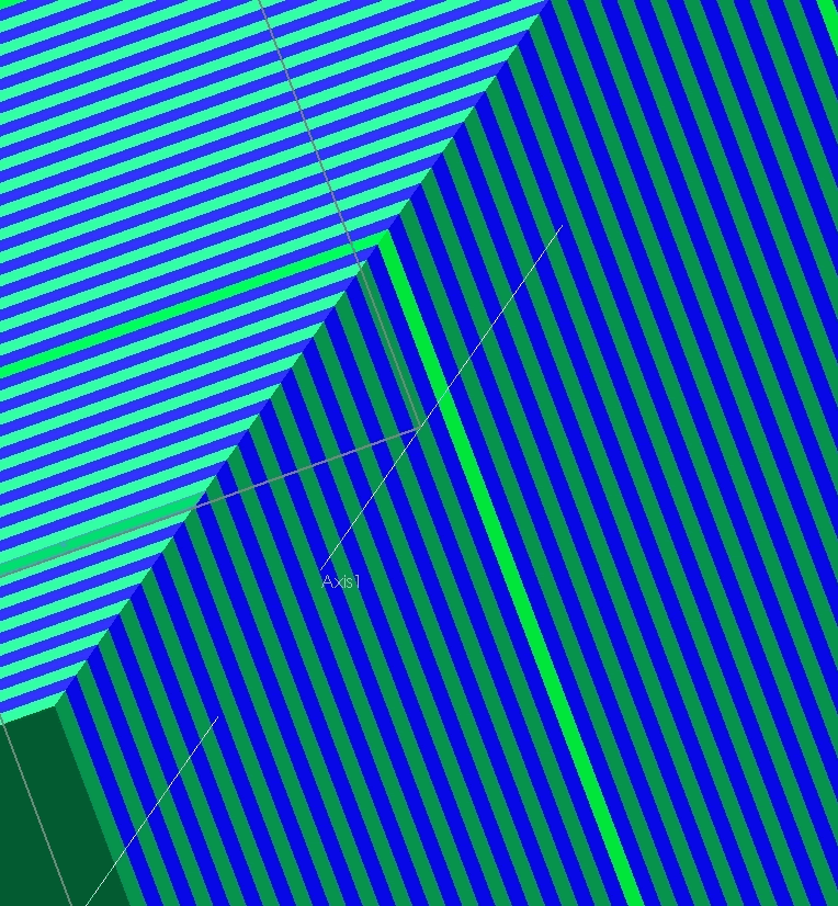
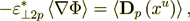
Figure 1: Two phase layered structure composite - superlattice of 100 layers with 50 layers each phase
Electrostatics Statement
Here is the problem with old and respected roots. The problem that can be called and used as the "litmus paper" - when we want to check, compare and control the main features we need to examine the problem which is clear in its statement and has a history of classroom work. The problem of distribution of electrostatic field in-cross (as well as in parallel) to the plain layers of two or more kind of materials is exactly a good benchmarking task. There is a constant flux of people returning to this problem. We have happened to solve this problem as the 2 scale problem. Fortunately, in a linear case statement it can be solved even analytically.
The first problem in scaled HSP-VAT electrodynamics (as well as in thermal physics) which happen to be solved analytically on both scales. Few results are given below.
This two scale connected solution, the solution that explains hidden in textbooks incorrectness's and
inconsistencies - it is supposed to overturn the many physical disciplines lecture courses. The main features of this solution and
consequences are known since 2003 - I also disseminated them to many professionals lecturing
in the universities, and particularly in fields demanding already for many years the usage of words - "multiscale,"
"averaged," "two scale," etc.
However, I doubt that these professors teach this new solution in classes. My guess is that they continue to use for this textbook incorrectly solved problem
the same old one scale solution and tell to students that in this way they can get the "bulk" transport properties!
But this is the false statement, because by this two scale connected solution shown inseparableness of different scale solutions and properties of the medium. First time by pure "in mathematics."
Unfortunately,
this situation is pretty much becoming close to what happened in Meteorology through the last 25-30 years when the wrong governing equations and
mathematics of the Upper scale equations have being taught to students through all these years. See our analysis and summaries on that in -
"Modeling and Averaging in Meteorology of Heterogeneous Domains - Follow-up the NATO PST.ASI.980064"
ABSTRACT AND FINDINGS
1) There are the exact solutions available for the lower (1st) scale of the 2-scale problem for the steady-state Laplacian equation fields applied in-cross for the 1D layered (superlattice) media. These solutions are given in textbooks on few physical disciplines (thermal physics, electrostatics, civil engineering, materials science, etc.) and often cited as to be the complete and final result.
2) The layers and their physical properties and thicknesses can be linear or space dependent, or nonlinear media.
3) As it was discovered recently that the Linear problems have the 2-scale Exact Analytical Solutions for the 3 kinds of Boundary Conditions: 1) field values (potentials, temperatures); 2) displacement or electric fields applied; 3) Neumann's conditions of the 3rd kind. The two-scale solution meaning the solutions on both scales - on the lower, conventionally adopted spatial scale; and for the Upper averaged fields scale.
4) The upper (the second) scale solutions are not achievable in brackets of homogeneous physics. There are no definitions and mathematics (at least correct ones) for that in homogeneous physics. That is why there is continuous search for experimental methods to measure the superlattice conductivity and dielectric permittivity. For example, most of the latest heat conductivity measurement methods use the transient try-and error fitting techniques to match the measured bulk data while solving the lower scale homogeneous transient heat conductivity equations. They calculate in this way the different - the TRANSIENT homogeneous bulk heat conductivity coefficient. That coefficient differs from a steady-state sought heterogeneous effective coefficient. Also, with these techniques there is no way to find out the Phase Effective Coefficients of conductivity or permittivity.
5) Because the solutions are available analytically for linear and with the help of numerical simulation for both scales nonlinear problems for this morphology of 1D layers, this is the unique problem to test and compare the both scales solutions. Up to these days () it is known as one of the first few kinds of such a problem solution in the HSP-VAT. Also allowing the analytical forms of the solution. There is no need to apply the word - "verify" to the upper scale solution, since there are few more the two-scale exact solutions have been achieved.
Figure 1: Two phase layered structure composite - superlattice of 100 layers with 50 layers each phase
6) The other problems of HS physics-VAT with the exact solution are - a) for a media filled with circular pores (or bars) and(or) b) with spheres embedded into a matrix or in a fluid with laminar flow. Those are more of theoretical interest and they have been already solved ( I can point out the references). The two-scale solutions are available to recognize at this site in -
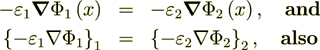
7) The dependencies outlined in homogeneous physics solutions are incorrect if being applied with the exact fields for the lower scale solutions as, for example, the homogeneous formula gives the displacement field in the system through the averaged electric fields (potentials)
and this value can be tens and hundreds times different from the correct one. We are
assuming here as usual that according to homogeneous Gauss-Ostrogradsky theorem
the following is true - the averaged  over the each phase 1, 2
gradient operator acting on the potential function
over the each phase 1, 2
gradient operator acting on the potential function  is equal to
 (1.1)
(1.1)which is incorrect, but anyway our goal is right now to proceed further.
8) The known "classical" formulae for effective coefficients can be calculated as known for bulk values only for linear problem. It is important to say that the formula for the linear effective bulk coefficient
is correct, but is not valid for the derivation! Final result and the formula is correct, but the derivation is not correct? It can not be derived even for linear problem when applied only one scale homogeneous knowledge base.
That is because 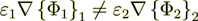 , in spite that the homogeneous fields
formula
, in spite that the homogeneous fields
formula 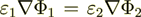 is correct and the local lower scale
 is correct also.
I supply below the direct calculations based on the exact solution which supports this statement.
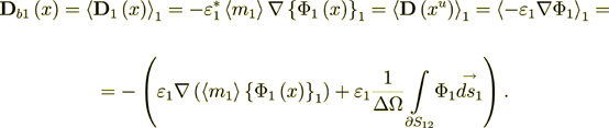
9) This particular layered morphology of the two-scale problem dictates the peculiarities of the physical phenomena involved. Thus, for the linear problem there are the two additional (to the known homogeneous one scale term(s)) physical mechanisms involved in the field's transport (steady-state) - 1) is the common knowledge Homogeneous INTRAPHASE, in each phase transport; and 2) is the INTERFACE transport (term(s)); and 3) is the INTERPHASE (between the phases) transport and term(s). In most common situations those are the three different components in the transport characteristics. The later properties described and accounted for as to the physical phenomena seems only in chemistry, chemical technology.
In electrodynamics it is still considered as the 3D phenomena of a one scale.
10) The calculation of two components of the interscale transport - the Intraphase and the Interfacial one gives the understanding and values of new phenomena in superlattice transport.
11) The mathematical formulation and exact calculation of the surficial transport components give an expected explanation of decreased overall bulk permittivities and what is more important is of their magnitudes. It also allows to compare transport in each separate phase along with their components.
12) Neddless to say, that the unknown component of interface transport can reach values of hundreds and even thousands percent of effective bulk values - see Figs. 2,3 below. That can be directed toward the explanation of some known physical phenomena as, for example, like the interface resistance and polarization among others.
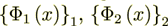
13) There are new phenomena verified by direct simulation for the "bottom- up" as well as for the "top-down" scaling connection of physical entities as, for example, I can find out the lower scale complete solution without solving it as it is known to be solved. All is based on the knowledge of the upper scale characteristics. The kind of interscale mathematical transform (IMT) or Top-Down Scaleportation, where the upper scale determines directly the lower scale properties.
This is the strict and direct evidence of communication of the physical properties on both scales, and this is one of new discoveries.
14) I supply below the algorithms and the numerical simulation results using the exact analytical solution for the lower scale superlattice in-cross electrostatics transport problem. It is given in terms formulated for the electric field strengths (displacement fields), but is valid perfectly and for the thermal physics conductivity problem as well.
THE ANSWER TO THE QUESTION AT THE BEGINNING IS AS USUAL - LET'S GOING TO ANOTHER SPACE (WHERE THE EQUALITY HAPPENS)
2.1 Problem Statement and Simulation
There is the system of k layers, layers are changing one after another
(intermitting); with  - dielectric permittivity of the odd layers,
 - dielectric permittivity of the even layers;
 - thickness of i-th layer;
 - coordinate of the boundary of the i-th layer;
 , where
  is the
layers pack's left boundary z-coordinate.
is the
layers pack's left boundary z-coordinate.
1) We consider the superlattice which is the heterogeneous medium of 100 or 200 or even bigger number (600+) of layers, consisting of homogeneous, with constant coefficients layers of two kinds, or inhomogeneous layers of two kinds when each layer of each kind has the inhomogeneous or nonlinear dependency (we consider here only this kind of equations, and not going to write down at this time here the all new equations of Maxwell-Heaviside-Lorentz (MHL) Heterogeneous Electrodynamics) for dielectric permittivity problems.
1 For the lower scale medium each layer of kind 1 or 2 we can write for the perpendicular applied electric field that for:
1) First period - two layers -
 (1)
(1)

and
 (2)
(2)

with the conjugate boundary conditions of the IV-th kind BC's like in thermophysics conductivity problem. The two fields are having at the interface surface the BC's, for example, when the phase 1 contacts with the phase 2, then
 (3)
(3)while the second BC appears as
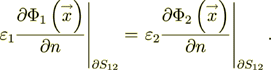 (4)
(4)And for the all other periods the same mathematical statement is valid.
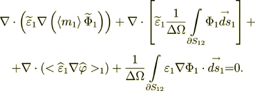
2 The Upper Scale VAT Governing Equations
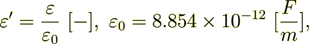
Meanwhile, when coefficient of conductivity
 , and permittivity
  ,
in the phase one then the VAT upper scale equation for potential in this phase is
,
in the phase one then the VAT upper scale equation for potential in this phase is
 (5)
(5)
(actually the same equation as for heat conductivity and mass diffusivity modeling, see: Travkin, V.S. and Catton, I., "Heat and Charge Conductivities in Superlattices - Two-Scale Measuring and Modeling," in Proc. 2001 International Mechanical Engineering Congress and Exposition (IMECE), IMECE/HTD-24260, pp.1-12, 2001; and Travkin, V.S. and Catton, I., "Analysis of Measuring Techniques of Superlattices Thermal Conductivity," in Proc. 2001 International Mechanical Engineering Congress and Exposition (IMECE), ASME, IMECE/HTD-24348, pp.1-12, 2001).
In the second phase we get the same kind of equation
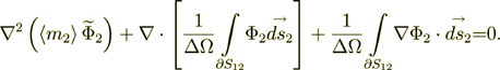 (6)
(6)
see more explanations and derivation of some Upper Scale MHL Heterogeneous Electrodynamics Equations in texts -
Introduction to Heterogeneous Scaled Electrodynamics ,
FUNDAMENTALS OF SCALING HETEROGENEOUS SCIENCE,
and other publications, part of them in -
References (mostly on Electrodynamics topics) .
The effective coefficient of permittivity for this heterogeneous media as a whole is
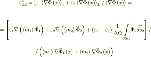 (7)
(7)which can be shown is to be reduced to the known formula
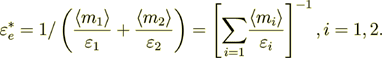 (8)
(8)Meanwhile, this formula is not applicable for inhomogeneous and nonlinear problems, for example, of this kind
 (9)
(9)
 (10)
(10)

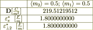
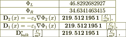
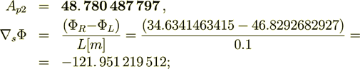
For the number of layers k =100, layers left boundary potential
 = UL =46.8292682927 [V], while
layer's stack right boundary is
= UL =46.8292682927 [V], while
layer's stack right boundary is  = UR =34.6341463415
[V], thicknesses are l1 = 0.001[m], l2 = 0.001[m], the coordinate of the left boundary is
= UR =34.6341463415
[V], thicknesses are l1 = 0.001[m], l2 = 0.001[m], the coordinate of the left boundary is
 = 0.001[m].
This is the part of the more general problem - that is why the Boundary potentials are not simple short numbers.
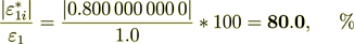
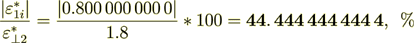
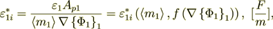
The effective dielectric permittivity coefficient  as shown above for
such a combined heterogeneous system (given in textbooks)
as shown above for
such a combined heterogeneous system (given in textbooks)
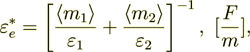 (2.1)
(2.1)here we designate
where 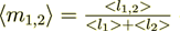 average volume fraction of the phase 1,2.
Meanwhile, the bulk medium electric flux density (displacement field) is found
average volume fraction of the phase 1,2.
Meanwhile, the bulk medium electric flux density (displacement field) is found
as
 (2.2)
(2.2)Tedious VAT derivation can be presented and leads still, for only constant phase coefficients to the known following formula
 (2.3)
(2.3)while the complications as, for example, the inhomogeneous phase coefficients, or internal charge sources, or additional interface resistance, or/and the phase's nonlinear data of input will get much more complicated formulae for the effective coeffcients.
Nevertheless, the mathematical expressions for effective coefficients have been derived explicitly (Travkin and Catton, 1998,2001), which means that the coefficients can be found directly. It is no secret that for the inhomogeneous, nonlinear problems of this kind there is no solution in the homogeneous physics. More of that, the Direct Numerical Modeling (DNM) results if appllied straight toward the derivation of the effective variables using formulae for homogeneous media give incorrect output as, for example, when calculating the derivative content
 (2.4)
(2.4)will give incorrect average displacement field, even when the source fields
 are known with high accuracy.
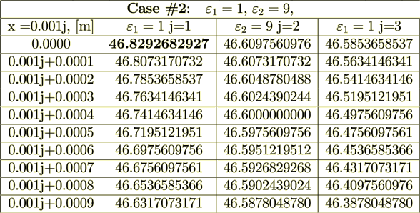
Case #2: Dielectric Permittivity Coefficients are rather different ( =1,
=1,  =9)
=9)
#2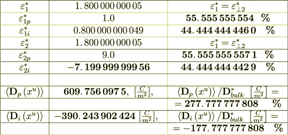
#2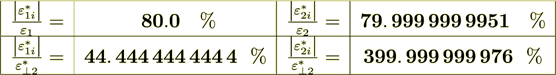
#2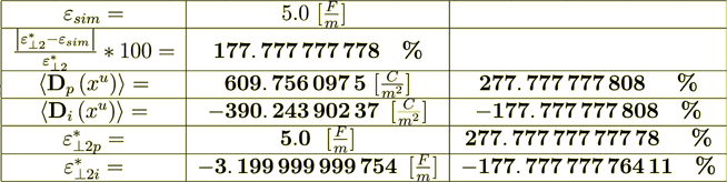
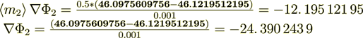
2.2 Homogeneous Physics Straight Simulation of Bulk Effective Permittivity -

As soon as

then following from homogeneous definition

and the further homogeneous formula gives
 (2.5)
(2.5) Not a close match to the correct  = 219.5121951
one can calculate
 (2.6)
(2.6)
So, they are not equal -
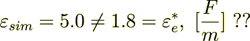 (2.7)
(2.7)the difference is
Quite different values then for the not so close coefficient values
, .
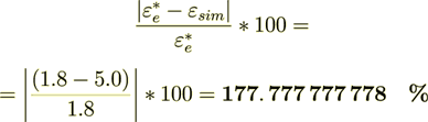
What is the result? Why is it incorrect?
When students had checked this before and to what idea they could come?
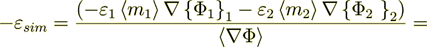
2.3 Heterogeneous VAT Simulation of the Data in Each of the Phases
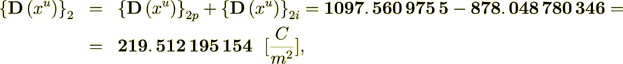
Now let we find the  of the averaged functions (or fluxes)
- this calculation for linear problem is good. Now the homogeneous "averaged" flux is

now checking the displacement field

So - this means that According to Homogeneous Physics this Could Not be the Truth
![]() How Could This Be??
How Could This Be??
2.3.1 because according to homogeneous physics for this problem should be satisfied
 (2.8)
(2.8)the two next equations should be fulfilled
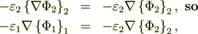 (2.9)
(2.9)but we have
 (2.10)
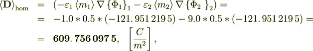
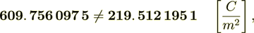
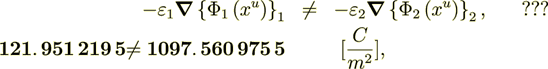
the difference is in the whole 7-8 times ??
even this stupid trick does not work: (1097. 560 975 5 -121. 951 219 5) /2 = 487. 804 878 =
so
(121. 951 219 5+487. 804 878) = 609. 756 097 5 not good.
That means also that the specific assumption for this morphology - is that the
averaged variables can be used in this equality (meaning that 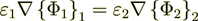 )to derive the effective coefficient formula when using
is not valid for the derivation!! Final result and the formula is correct, but the derivation is not correct?
Because  , but the homogeneous
 is correct and
  is correct also.
A-yah! What does this mean?
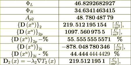
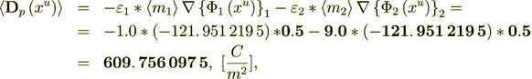
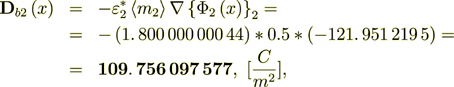
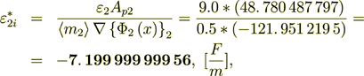
Calculating the VAT based surficial (Interface) integrals using the lower scale exactly calculated fields
 (2.12)
we got the value for current input data and the solution calculated as

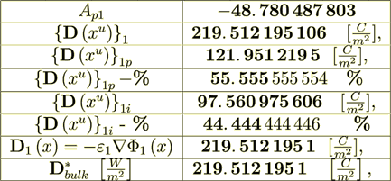
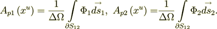
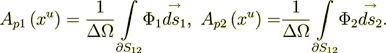
Symmetrically we can get the Ap1


Now I can calculate the variables in the phase 1 as -
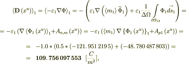 (2.13)
If only take the gradient part of the flux which is the Intraphase component then we have

while the interface surface component is

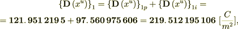
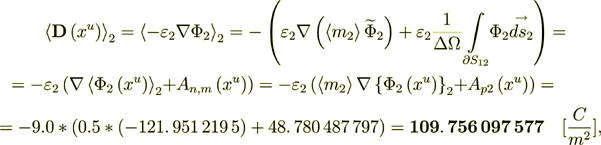
The whole averaged over the Phase 1 heterogeneous Upper scale displacement field is

:  where
where  is the intraphase transport part,
while
is the intraphase transport part,
while  is the interface transport component.
This Upper scale electric density flux is Pretty well coincides with the lower scale flux - so, the energy balance is perfect!
Now - calculate the intraphase transport phase only related part
 (2.14)
: 121. 951 219 5 
55. 555 555 554 %
At the same time, the surface transport part occurring only in this phase is
 (2.15)
: 97. 560 975 606 
44. 444 444 446 %
Checking the balance
 (2.16)
That is the balance of different electric field components.
For the phase 2 calculations show the same characters of numbers
 (2.17)
If only take the intraphase gradient component consisting then we have

while the interphase surface part is

If I would use the only formula homogeneous lower scale displacement value - I get this

and the heterogeneous scale internal phase two displacement field is the same
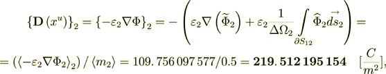
Where also  where
where
 is the phase transport part, while
 is the interface transport part.
This Upper scale
electric density flux is also Pretty well coincides with the lower scale flux - so, the energy
balance is perfect!
is the interface transport part.
This Upper scale
electric density flux is also Pretty well coincides with the lower scale flux - so, the energy
balance is perfect!
Now - calculate the intraphase transport part
 (2.18)
: 1097. 560 975 5 
100 = 55. 555 555 557 1 = %
At the same time the surface transport part is
 (2.19)
Percent is

= 9%
That is the balance of fluxes is perfect
While the Lower scale homogeneous flux equality is perfect - (the exact solution)


The internal stack's homogeneous formula electric density flux is
Meaning that the balances of displacement field in the two scale VAT approach are perfect for all the scales and for effective coefficient statement problem!
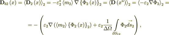
2.4 Heterogeneous Upper Scale Displacement Fields in Terms of VAT
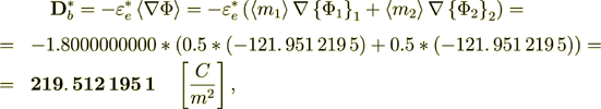
Now - let I do the calculation of the right hand side for the equation for effective coefficients modeling and simulation in this medium
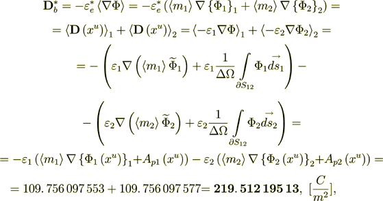 (2.20)
where as we defined
 (2.21)
To combine the components of the intraphase and of the interphase field's components separately we get
which is grossly out of touch for explanation.
And this is the very important result - Meaning that the Combined Homogeneous Density Fields - ARE NOT EQUAL TO THE PHYSICAL Fields?!!! JUST NOT EQUAL!! BALANCE IN THIS EXACT SOLUTION PROBLEM IS NOT COMPLETE IN HOMOGENEOUS PHYSICS!!
But when we use the surface transport Components as the VAT indicates to us we got the complete satisfaction with numbers
 (2.23)
 (2.24)
: -390. 243 902 424 -390. 243 902 37 :The difference is the result of numerical approximation, I believe.
Now do the percentage -

while the surface transport represents as

So, we see that this percent is very High in this variant. The right hand side BALANS IS
 (2.25)
: 219. 512 195 076 Is Perfect; - these are the displacement fields as they should be in any scale, and also this demonstrates the amazing accuracy of all calculations.
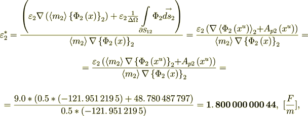
2.5 Heterogeneous Upper Scale Dielectric Permittivity Coefficient Components in Terms of VAT
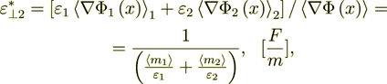
Taking the equality
 (2.26)
where the left hand side is assumed to be written in homogeneous definitions, while the right hand side in heterogeneous ones we can get the intraphase component of effective permittivity as it understood in homogeneous physics as following
 (2.27)
 (2.28)
or it appeared that
 (2.29)
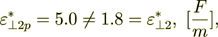 (2.30)
Now, the second component of the effective bulk permittivity is
 (2.31)
 (2.32)
Now we see that their sum is exactly equal to the composite's effective permittivity coefficient

Now do the percentage -

while the surface transport represents as

The same percentage as with the displacement fields component values - yes, the same.
2.6 Heterogeneous Upper Scale Resistance Coefficient Components in Terms of VAT
If to consider this problem as for the effective conductivity across the stack of two phase layers then we can find the bulk resistivity of the stack.
The specific intraphase resistance of the stack's medium will be
 (2.33)
while the interface component of resistance is even higher
 (2.34)
Or expressing this in units for the whole superlattice stack resistance we have for components
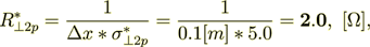 (2.35)
 (2.36)
For the total effective specific resistivity coefficient I can write
 (2.37)
 (2.38)
or in the device units
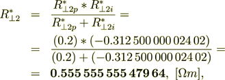
they are equal.
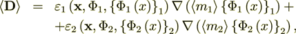
2.7 Calculation of the Each Phase Effective Coefficients in Terms of VAT
We know that

and can equate the both parts - the left one which is written in homogeneous notations and definitions, and the right one which is based on the heterogeneous medium determined mathematics, for the purpose of finding the Phase Effective Coefficient
here in the left side I used the nomenclature from the homogeneous physics, because we calculate the effective coeffcients for homogeneous - unusual, but homogeneous equation.
From this equality here I can get
 (2.39)
 so in this situation with linearly determined phase values, 
 (2.40)
 - it coinsides with the 
Now let I do the value of influence - present the phase effective coefficient as
of the two parts - intraphase  part and the interface surface
influenced coefficient component
part and the interface surface
influenced coefficient component  .
.
 (2.41)

 (2.42)
Now do the percentage -

while the surface transport represents as

In this variant the percent of interface influence is rather high. Also it is interesting that
 (2.43)
 (2.44)
 (2.45)
We knew that. So, the interface transport input to the phase 2 effective coefficient of permittivity is equal to
 (2.46)
for this problem it will be the component not dependent on spatial argument in this particular problem. But generally it will depend on coordinates and other arguments.
2.7.1 Doing the same for the Phase 1 effective permittivity coefficient estimation:
Homogeneous

again I can equate the both parts for purposes of finding the Phase Effective Coefficient
 (2.47)
Here I used the nomenclature of the homogeneous physics, because we calculate the effective coefficients for homogeneous - unusual, but homogeneous equation.
From this equality here we can get
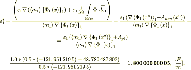 (2.48)
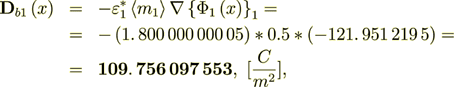 (2.49)
 - the same value as through the Phase 2 and equal to averaged value

Now let I do the value of influence - to present the phase effective coefficient
as of the two parts - intraphase  part and surface transport component

 (2.50)
also equal to the bulk phase permittivity coefficient, while the interface component is
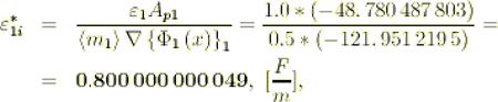 (2.51)
 And we see, that the interface permittivity component in the phase one (1) is not equal to the
interface component in the phase two (2) !!
 (2.52)
Now do the percentage -

while the surface transport represents as

Also it is interesting that
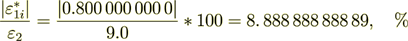 (2.53)
 (2.54)
 (2.55)
The same percent as for the Phase 2 fields.
We knew that. So, the interface transport input to the phase 2 effective coefficient of permittivity is equal to
 (2.56)
for this problem it will be the component not dependent on spatial argument in the problem, while for general problem statements it will depend on all arguments shown above.
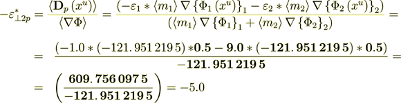
Few interesting relations between the permittivity in-cross coefficients for superlattices
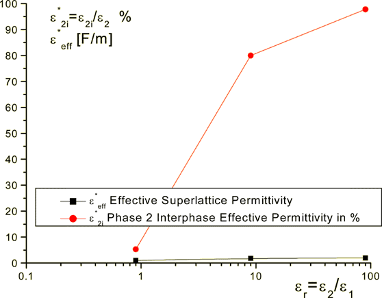
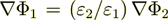
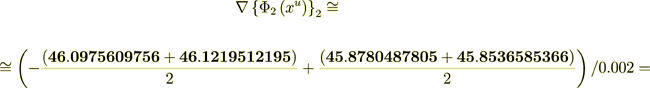
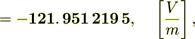
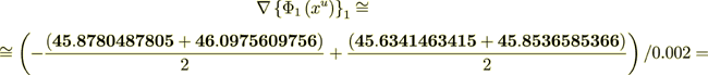
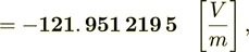
Figure 2: The effective coefficient of permittivity for the superlattice of 100 layers and the 2nd phase interface permittivity component relative value
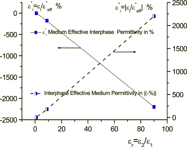
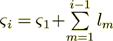
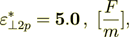
Figure 3: Medium's nondimensional interface effective coefficient of permittivity for the phase 2 of superlattice with 100 layers - the real and the absolute relative values
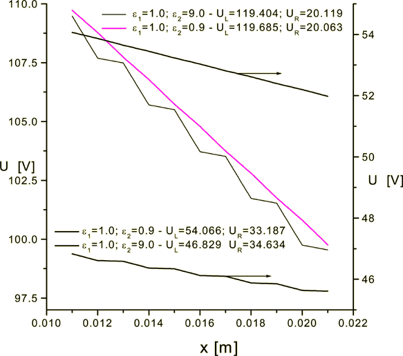
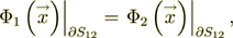
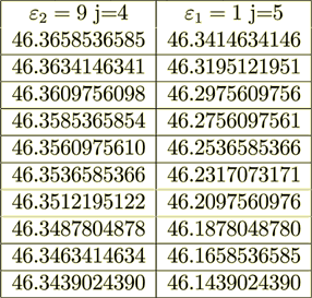
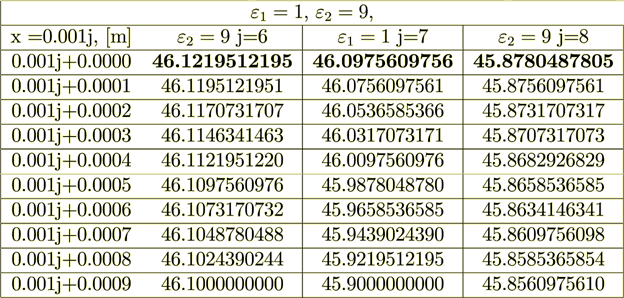
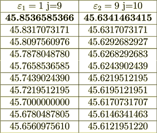
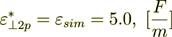
Figure 4: Potential across the superlattice for 4 variants with different ratios of dielectric permittivities and potential drop