When a heterogeneous medium (as the URL, in Meteorology and Urban Air Pollution) is the subject for experimental set-up and consecutive data reduction methods, then it is that the problem with the naturally physically seen two (or three scales if buildings interior is the conjugate medium as well) scales of phenomena in action. And when these problems being approached with the standard set of Homogeneous one scale fluid mechanics judgments, then we see the difficulties with assessment of what are considered as the results - the fields of meteoelements and pollutant concentrations.

Contrary to the Homogeneous medium treatment, if one would be able to use the two scale transport (and interests) VAT concept and modeling tools, then the results are capable to model the problem as the two scale one - even with the parametric inclusion of few effects. Note, that many features are not just available for the one scale - one or two-phase simulation.

For example -

1) The inclusion of morphology properties directly into modeling equations is available and mandatory for the VAT models. The experimental features of heterogeneous media (URL or vegetation) became available and immediately tied directly to the physical and mathematical VAT two-scale model.

2) The modeling coefficients are directly tied to the physical and morphological properties of the task - following the specifics of given URL's.

3) There are features of transport between the street air qualities and the buildings (second phase) air quality. More of that, when the internal buildings pollutants sources introduced into the third medium model, the level of concentration inside of the buildings can become much higher then of the street level. This experimentally found feature is not properly modeled when the only buildings air pollutant concentrations simulated as in a separate phase system. Those two spatial environments are conjugated media. And these are special features dramatically different for the medium of street air and the building's interior space. By the way, mostly the population provides the time spent within the buildings, so, this is much more important task to model and analyze.

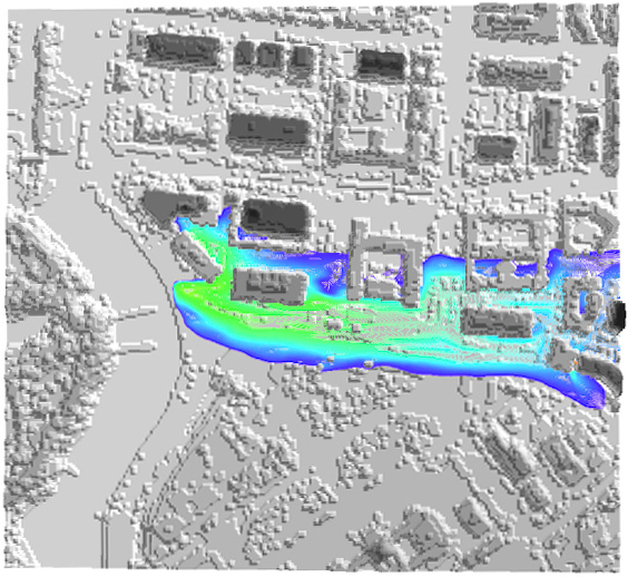
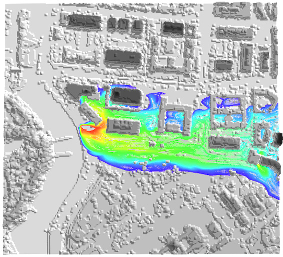
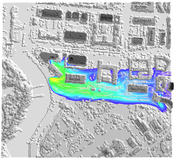
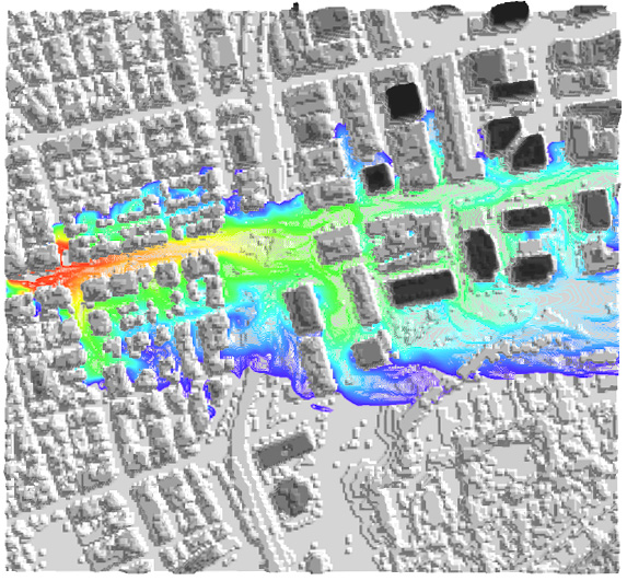
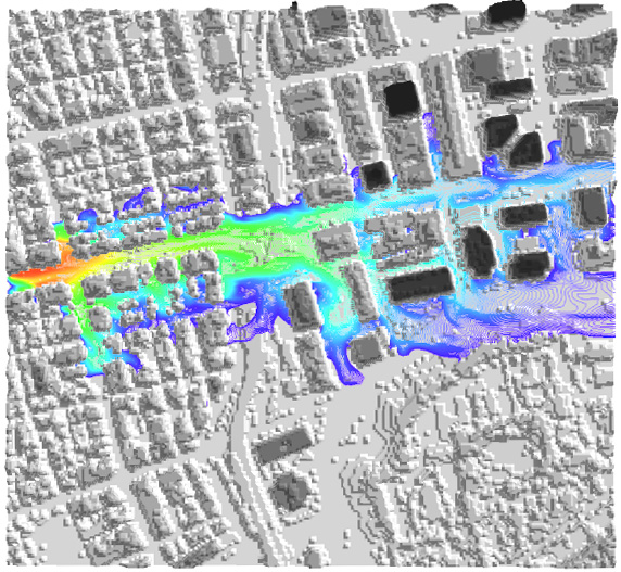
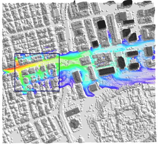
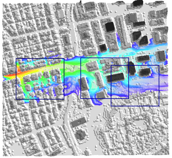
4) The output model's data - even for one scale Homogeneous Models the results should be presenting the values of some representative volume (REV) or some of the substantial domain within the problem's acting volume, which is the final goal for the assessment of hazardous situation. Otherwise, as we illustrate below, the local concentration of pollutant's field SHOW NOTHING BUT JUST Concentration Level at given point(s). This kind of output results show nothing useful, but the spots of instantaneous maximum concentrations. These points of maximum concentration will be sneaking to another spots depending on the wind direction and other external meteoconditions. To make things more obvious I would say, that in this mode we virtually demonstrate the instant flow field and the pollutants concentration fields around of one and few sand grains in the sandy beach and asking for the permission to lay down the resort? Does it have any sense?

On another side, should be the Local Data simulations treated with some special kind of volume averaging procedure following the VAT specifics, then the all two-scale features and characteristics as, for example, concentration fluxes calculation following averaging procedures calculation would be available. They will be simulated incorrectly if using the homogeneous GO theorem, etc. We have shown this for technical scaled problems, which are easier undergoing physical and simulation experiments.

More on the one scale features. Using the one scale simulation results:

5) Can the authors of experimental studies (and numerical simulation) assess the Reynolds number? Not a local point Re number, but characteristic one for the medium as the heterogeneous non-local entity? Or any other characteristic nondimensional number? I can not see this in any of these experiments or high definition DMM-DNM the standard fluid mechanics parameters ?

Why ? Because authors of one-scale studies just don't know how to make them up ? Locally - it doesn't have any sence. Some kind of Bulk Value - then, How to justify and calculate those ?

6) Someone can not calculate the rates of concentration wash-out, because the mean fluxes in any direction unavailable to calculate correctly in one scale homogeneous statements.

7) The rates of fluctuation in the contaminated areas are not available - because the instant local fluctuations as shown in many figures are just instant characteristics not useful for the health threat assessments.

8) The rates of concentration exchange between the street level air and the buildings internal space structures air are unavailable.

9) The rates of adsorption in the contaminated areas are not available; etc., etc.

To illustrate the issues I have written above I would like to use few studies from the NATO AS-980064 Institute - Kiev, May 4-15, 2004 and from some other investigations.

The studies concerned with are the physical experiments and the numerical simulation experiments.

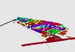
These pictures below are from the report by Coceal, O., Thomas, T.G., Castro, I.P., and Belcher, S.E., "Turbulent Flow Over Groups of Urban-Like Obstacles," in NATO Advanced Study Institute-980064, Institute of Hydromechanics, Kiev, pp. 62-63, 2004.

can be found at - "Coceal/", 

and we need to continue the talk about this report started above in "Modeling and Averaging in Meteorology of Heterogeneous Domains - Follow-up the NATO PST.ASI.980064" -

This is the very much awaited study - with the simulation experiment aimed to calculate the some part (stress tensor components) in the averaged Upper scale equation of turbulent momentum for inside and above the porous layer. The porous layer was taken as the regular network of straight square pin fins.

The authors did attempt to make averaging of the flow dynamics characteristics as the Reynolds stress in usual sence, and of the dispersive stress one component (vertical) as via using the equation (following Raupach and Shaw, 1982)
with the spatial fluctuation given as
where the averaging done as the surface-plane 2D averaging
This momentum averaged equation is incorrect equation - see the analysis above in the http://travkin-hspt.com/urbp/turbpart/Turbpart.htm

As I said, I consider this is the good experiment, with errors but still a good experiment.

Furthermore, admitting that we had put the large number of terms into that function , the value of is undermined because of the type of averaging - the 2D surficial, plane intrinsic phase surface averaging. And this is the reason why the curve for "dispersive stress" is rather small in values in the region filled with pin fins, and the Reynolds stress curve is so unusually straight-strong above the pin fins. The "dispersive stress" curve I think ought to be much larger in the pins volume and above it for some extent. Or the local turbulent fluid stress should be smaller in the region of pin fins.

There is the problem with calculation of morpho-fluctuations and the instant value fluctuations.

Also, because the problem's momentum equation formulated with incorrect averaging - the balance of "stress" tensor different components as it was performed for these two terms incorrect because of the sharp change in the fluid fraction in the REV, even in the 2D REV. This is the one of situations (problem's morphology) when we have the boundary between the homogeneous fluid volume and the two-phase "porous" like domain. The vector (tensor) fields should be continuous through this boundary, meaning we need the Phase Averaging, but not the Intrinsic Phase Average of the velocity field.

Also, there might be a problem with the uneven shape of the 2D REV authors had chosen to perform averaging over it. The computational domain seems was the same as the REV averaging in plane, and this is the problem because that 2D REV would be asymmetrical in x,y plane.

The Figure 2 on page 63 (also seen above) is incorrect - because of averaging type used and incorrect equation itself . Specifically - few moments we would reiterate here for the clarity of arguments and to return to basic definitions. I need to say again that the inconsistent (with broken derivations) application of the VAT theory, when researchers try to reinvent what has been written many years ago and very much known in other disciplines, bring down the incorrect governing equations, creates confusion and loss of time.

Authors noted that - "Averaging over shorter timescales gives significant dispersive stress even above the array." This is the correct comment and more on that - this is the correct intension, if any to make the dispersive "stress" (here it was not completely defined) larger. It should be larger due to number of reasons, at least two of them I would mention here - a) that the averaging should be provided over the finite volumetric slice, but not a plane surface as done in this study; b) morphology related fluctuations stress function derived using the intrinsic phase average, of coarse is incorrect.

Also, I would easily argue that there is no balance of momentum on the Upper scale confirmed through the usage of this "averaged" momentum equation.

The determination of the Re number presents a challenge in this kind of formulations.
~~~~

Returning to the study by Pokrajac, D., Cambell, L., Manes, C., and McEwan, I., "Interpretation of PIV Measurements of Open Channel Flow over Rough Bed Using Double-Averaged Navier-Stokes Equations," in NATO Advanced Study Institute-980064, Institute of Hydromechanics, Kiev, pp. 156-157, 2004,

I would like to comment here in this subsection because in this study the same kind of research aimed to calculate based on experiment the morpho-stress term

in the almost correct (one term absent) momentum equation

When they took the morpho-stress term in the form shown above as in the momentum equation - by this form alone they almost disintegrate the influence of the very important variable morphology function - the porosity function. This action was done specifically to eliminate the influence of porosity function - and this is mistake. It appeared later, that the morpho-stress and the turbulent stress related terms have almost no connection to the porosity function - but this is the opposite situation according to the morphology models of the both these close by like "design" studies.

That is why we see here so strong jumps in stress curves at the height of the obstacles - there is no conservation of the tensorial variable's fields.

As long as the specifics of the averaged domains are not available from the lecture presentation's slides at this moment, and the "stress" curves behavior reminds closely the same curves I commented above regarding the calculations by Coceal, O., Thomas, T.G., Castro, I.P., and Belcher, S.E., (2004), my guess would be the same - that there were taken the 2D averaging flat horizontal domains for calculation of the morpho-stress in the lower layer occupied by "porous" medium

The closure techniques and the peculiarities of the volume averaging integration should be disclosed by any research team - to make available for others in the community to make a judgment. That's according to our experiences. This is the same situation as with the physical direct measurements - when ONLY THE EXPERIMENTALIST IS NOT SURE ABOUT THE RESULTS, although the outside reader tends to believe to experiment more than to the theoretical results ? To the theoreticians it remains a mystery - Why is that, because we know about numerous reasons the experimental study can show wrong tendencies?

That is why journals demand usually from authors of an experimental work the features of the applied measuring techniques.

And this is exactly the cause I am talking about: the data reduction for DMM-DNM or direct physical experiment for these VAT two-scale tasks are not so obvious Homogeneous physics data reduction routines as are being used right now by this small number of groups who actually sensed the taste for these problems in meteorology and pollution modeling! !

As I said above - that there is the problem with regard of the procedures how researchers will calculate the morpho-fluctuations and the values of instant fluctuations.

At this stage of the two scale VAT turbulent research we are at the similar situation - when the many details every team could develop for themselves should be verified by others when doing the analogous operations.
~~~~

Finnigan, J., "Turbulent Flow in Canopies on Complex Topography and the Effects of Stable Stratification," in NATO Advanced Study Institute-980064, Institute of Hydromechanics, Kiev, pp. 20-24, 2004.

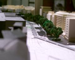
The picture below is a fine demonstration of huge effort researchers do to study the subject.

In spite that this is the two scale problem, the goals for this particular experiment were stated as for the one scale specifically difficult turbulent process mission.

We are familiar to this kind of measurements. This experimental set-up for meteorology study happens to be close in mechanical design to the one we used for similar goals for problem in semiconductors heat sink devices design.

In our study we were concerned with providing the two scale measurements - the local and the bulk, "averaged" in some fashion according to the VAT requirements and to the available resources. In that way we found the great increase in amount of workload, measurements sampled, quite different data reduction needs and similar problems. Partially due to this significant enlargement of labor and time restrictions, that study was not done as an accomplished one. Anyway, a number of problems had been solved and results with two scale measurements of this kind can be seen at -

Finnigan, J.J. and Shaw, R.H., "Large-Eddy Structure and Low Dimensional Modeling of Canopy Turbulence," in NATO Advanced Study Institute-980064, Institute of Hydromechanics, Kiev, pp. 80-81, 2004.

This experimental set-up below according to its title is supposed to measure the velocity covariance function - as a lower field point measurement function, in the dense simulated vegetation canopy layer. What we get in here is the unusual covariance function, no questions. The next thing to do is to understand what is this?

If this is the function which considered as just a turbulent two-points special medium function as we know it - then where are the special medium properties in here ? Where is the special medium second phase vibrations feature? But even when vibrations are absent in the canopy as it is in the experiment shown above, then to take these multipoint measurements as the two points straight line distance in between function is an illusion.

We can not throw away the second phase presence and the boundary layers over its surfaces, etc. etc.

The next three figures are the illustrations from the report by Amorim, J.H., Miranda, A.I., and Borrego, C., " Air Pollutants Dispersion Disturbance Due to Urban Vegetation: a Porous Media Modeling Approach to Lisbon City Centre," in NATO Advanced Study Institute-980064, Institute of Hydromechanics, Kiev, pp. 46-47, 2004.

In the first slide compared the concentration fields for the same area around of the main street with and without the "porous" medium of trees. First of all, the pictures are very nice looking, but asking ourselves what is(are) the characteristics we can measure and compare beside the color - meaning absolute dot-concentrations? We can not answer to this question being inside of the one scale point-concentration and meteorology elements physical and mathematical statement. Everybody familiar with methods used in chemical technology modeling, mass transfer science knows that having the distribution of fields in the problem domains says nothing useful, but some general observations. No quantitative assessment can be delivered into the data reduction, unless the methods of data reduction and nondimensional analysis taken as tools. But what kind of non- dimensional characteristics we can take and calculate here ? The one scale model does not have answers to this. Well, not exactly as we will talk below about statistical methods of data reduction.

Another point, regarding this picture is that the vegetation areas are known as generally to be very much helpful in cleaning the environment!

In this modeling case here - with like "porous" vegetation volumes had been taken into account - we see that results are opposite - with the vegetation volumes in place the concentration level is raised significantly? My guess would be, that something wrong is with the model itself? With the way the "porous" volumes of vegetation were incorporated into the One Scale Lower scale mathematical model.

One of the useful procedures in this case is the total check of the conservation within the problem's domain? Whether the raise of the concentration in sub-volumes is within the total amount of pollutant component or its volume is not in balance with the initial amount of pollutant? The volume integration is inevitable anyway.

The next point - is the measurements, taken in the area of simulation. But these can not be compared with the current method of simulation. The measurements were taken as an almost dot local measurements - the measuring booth is the small scale device and the sensors array is of the small size either. The time scale of the measuring point is about of few minutes. On the other side, the volume of unit grid used in the simulation is of the tens and hundreds cubic [m^3] meters. That should be a special care taken of regarding these comparisons.

The following below is the picture where the buildings' surfaces are of unusually high concentration of CO.

The buildings surfaces are also known as adsorbing surfaces. The shown on pictures the buildings external surfaces with this high inhomogeneous concentration tell about the two things: 1) is that the mass transport boundary conditions, probably, should be corrected, if not, and everything is correct with the local adsorption rates (if any taken into account); 2) then the mass transfer over the buildings surfaces is the real subject for accounting. And that can not be done in this problem using only the local dot-point mass transfer model.

The following picture is an example of an attempt to calculate some averaged values - in this case the plane surface averaging, if I am correct? The well meant calculation, still not enough to assess the needed averaged values for analysis and data reduction.

The next five figures are the illustrations from the report by Nakayama, H. and Tamura, T., "LES Analysis of Fluctuating Dispersion in Actual Urban Canopy," in NATO Advanced Study Institute-980064, Institute of Hydromechanics, Kiev, pp. 144-146, 2004.

Authors had generated impressive figures for the 2D concentration distributions in the two areas of Tokyo as results of the Lower level (scale) 3D DMM-DNM simulations.

The Kasumigaseki region characterized with the three pictures of different statistical slices (characteristics) -

and the Kanda area simulation using the same statistical selections (it does not matter for our analysis in what particular range fell the concentration field's selection arrays)

While observing the concentration fields up here in these two areas simulation the same question on adsorption modeling in the Urban Rough Layer buildings environment area comes to mind. In close to buildings vicinities we do not scrutinize, at least visually, the attenuation of the concentration field by buildings as the porous mass adsorbers.

So - with this data reduction model we even can not say with determination - What is the vertical range of this or that concentration shown in any picture? And this is the range from ~0(10m) to a few hundred meters? We can not assess the Health Threat to the public due to this or that specific situation! We can not answer questions from the city's authorities - To what features we should stick to in decision making regarding the Hazardous Situation? Because we had not calculated them, and we don't know What to calculate as the General Objective Characteristics? Not to the level of red color - that information is too lacking for the decision making. And besides, this color can change every 5 minutes?

I would modify slightly the subject pictures for the Kanda's area to the extent of showing the 2D Hypothetical region for the Upper Scale assessment of concentrations and other, including meteorological, fields.

The 3-rd dimension of the slice and the mutual arrangements are tightly dependent on the properties of the VAT simulation model.

The following few figures are the illustrations from the studies made at the Budapest University of Technology and Economics by the scientific team (see -

and Lajos, T., Szepesi, Z., Goricsan, I., Regert, T., Suda, J., Balczo, M., "Wind Tunnel Measurement and Numirical Simulation of Dispersion of Pollutants in Urban Environment," in Proc. Conference on Modelling Fluid Flow (CMFF'03), The 12th International Conference on Fluid Flow Technologies, Budapest, Hungary, Sept. 3 - 6, pp. 1-8, 2003,

also at Regert, T., Lajos, T., Csecs, A., Goricsan, I., Balczo, M., "Dispersing Urban Pollutants in Budapest," FLUENT NEWS, Vol. 13, Iss. 1, p. 17, 2004 )

The area of new City Center construction effecting the air pollution in the middle of Budapest

was the study goal. The research was done by physical experiment using the large wind tunnel facilities and by

numerical simulation also using the 3D area's buildings and environment spatial model for the FLUENT simulator.

The results of 3D numerical simulation presented here are for two different wind directions. In Lajos et al. (2003) it is explained that these 2D pictures are the 1.5 meter high above the ground level plane 2D cross-sections fields, "Fig.9. where the dimensionless concentration distribution is shown (simulated with Fluent) in a horizontal plane 1.5 m high above the ground, after construction of City Centre."

That is why these pictures are rather different from the concentration fields in Tokyo above.

It's of no surprise that in both studies researchers came to the statistical analysis of the field's results as to the only reserve. Below are given two figures from the same thorough study by Lajos et al. (2003) where the analysis done by comparison of the 4 experimental and simulation runs in the same points of the URL study domain.

Meanwhile, the 3D simulated fields of meteoelements and pollutant's concentrations are the gold data mines. The only thing authors of the Lower Scale DMM-DNM simulations needs is to use those data for the Upper scale simulation and get the thought after answers to the Logistics Questions they were asked by authorities before getting the financing.