Urban Experimental Morphology for the Urban Bi-Porous Air Pollution Three Scale Modeling

As one can easily imagine that the kind of urban surface seen in the following picture which is an ordinary scene for the urban center developed regions (downtowns) and which can not be considered or represented via the artificially elevated (earth surface followed) shell demands the 3D physical representation - the volumetric structure which at best would copy the reality of URL.

But the goal is not just to copy the spatial urban structure and to model the morphometry and the physical processes within an URL. The goal is to make the construction of the model (physical and mathematical) which helps to make the generalized analysis and conclusion on the higher hierarchy scale, as is what to say for comparison - the one atom or nanodevice physics, their models and features are of no representative interest toward the aim of designing the piece of material or process involving millions of nanoparticles to be combined in some fashion. But contrary, the both scales physics (well, roughly speaking, if to take into account only the two lenght scales) are responsible for matter's properties. Saying simply, that the contamination of an air in the one room in a hotel is not the conclusive and reputable basis to evacuate the hotel or the whole group of hotels in this neighborhood. The same token, the one accident of harmful or poisonous agent release on the street level few blocks from the White House might be not the reason to evacuate the White House.

The most close to the authenticity of the URL's Upper Scale physical model is the specific porous layer open from above which has the Three Scale double porosity features of the medium. The lowest spatial scale is the internal (room size) scale within the buildings environment. The next in size is the scale of buildings and of the street channels porosity, with the Upper scale being the scale of the URL or of the ABL considered if the horizontal scale is substantial.

  Urban Roughness Layer Morphometric Analysis

   The technique for obtaining a mathematical description of such an URL 3D surface-structure with a randomly nonhomogeneous roughness layer has been elaborated in 1980-82. The technique was different from the few known at that time methods and is based upon the analysis of morphometric characteristics obtained in the so-called elementary statistical volumes (ESV), into which the urban roughness layer is divided. Afterward the experimental morphometric data can be used in the URL volume averaging theory models.

     The method is particularly suitable for the experimentally verifiable or measurable urban roughness layers characteristics those in which the profilograms are not simple convex or concave curves, but differ in descriptions of curvatures and derivatives, and which are characterized by repeated crossings of normals to the subsurface and by the fact that the vertical dimensions of the nonhomogeneities (obstacles) may be of the same order or greater than the horizontal ones.

 Morphometrical data in one of new built-up area in the city of Kiev were analyzed (1980-82) with the aid of a specialized set of programs for morphometric processing and simulation of experimental data of the URL. Among the morphometric characteristics of the distribution densities to be calculated and evaluated were the distribution densities of surface and volume porosities, of distances between the obstacles and their granular composition, of heights and specific surface of obstacles.

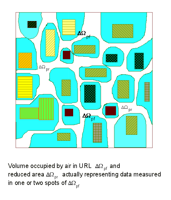
   The urban roughness layer turbulent transport VAT models offered incorporation of the not general, but strictly experimental allowance for the morphological characteristics of the randomly nonhomogeneous roughness layer of specific urban housing systems and phytocenosis and made it possible to assess their effect on the characteristics of the turbulent boundary layer and diffusion of harmful impurities in the urban roughness layer.

3. Urban Air Pollution Conjugated Two Scale Dispersion Models and their Closure in the Urban Rough Layer

The first step is to derive a set of volume averaged conservation equations from a set of turbulent transport equations. These equations are then made dimensionless by choosing an appropriate set of scales. Models for the turbulent mixing length, drag coefficients, and mass- and heat transfer coefficients are then developed to complete the model.

3.1 Lower Scale Turbulent Transport Equations

The averaging procedure starts with the turbulent transport equations

The closure of these equations requires a turbulence model to evaluate the Reynold-stress terms. A commonly used model is the turbulence model. A version from Rodi (1980) is

also

where

and P is the production term and is the buoyancy production (or destruction) term

Starting from this set of equations, different approaches are available for computing flow over rough surfaces. Mathematical statements in most published works describe the selected roughness elements in a way that depicts morphology characteristics serving as external restricting parameters either as boundary conditions or through the determination of a specific domain of interest. In a number of experimental studies (Perry et al., 1969; Lion et al., 1993, for example) and in a number of theoretical works (Tani, 1987; Kader and Yaglom, 1984), the friction velocity and shear stress are assumed to be measured at the "wall" level. What this means, is that is actually assessed or measured somewhere in the bottom part of the logarithmic velocity profile. This issue, not widely recognized, is the basis for most rough surface investigations. The distance from the wall for a rough surface is needed for each specific case of roughness morphology. For example, in a tube, the friction velocity and wall shear stress are

yielding the crucial quantity without real measurements near the wall.

The distance from the wall for which the shear stress concept has meaning should be of interest. The uncertainty in the wall shear stress height partially explains the appearance of additional terms in roughness surface logarithmic velocity laws. Thus, Nikuradse's law of the a rough wall (2) for a fully rough regime has an additive constant equal to when the dimensionless coordinate (70 or 80). Webb et al. (1971) dealt with this by using specific dependencies for the roughness function . The fact that in a fully rough regime, the drag resistance coefficient (friction factor) becomes independent of the friction velocity suggests that there should be correlations for each specific roughness morphology and channel type.

Youn et al. (1994) used numerical analysis to produce a correlation for the square rib roughness friction factor in a rectangular channel. Meanwhile, Liou et al. (1993) suggested a heat transfer coefficient correlation which reflects the impact of morphological parameters such as rib height and pitch on the average heat transfer for square ribbed roughness.

3.2 Volume Averaged Governing Equations

To make this portion of text more consistent I preserve here few VAT turbulent equations of general interest (those were already given in this and other sections of the website) for downroad development.

To use the concepts of the two scale medium transport VAT equations the Urban Rough Layer was dealt with as a heterogeneous porous medium. This method was based on the theory of averaging the turbulent transport equations in the REV developed in 80-th (Scherban et al., 1986a; Primak and Travkin, 1989).

The horizontal dimensions of the REV are far greater than the characteristic dimensions of the roughness elements in longitudinal direction. In the case of regularly arranged roughness elements the longitudinal dimension of one REV is typically one pitch of the roughness elements.

After averaging the basic initial set of turbulent transport equations over the REV and using the averaging formalism developed in our previous works, one obtains the following equations for mass conservation

for turbulent filtration. Momentum equation with penetration through interphase surface (as, for example, the building wall) has the form

In this equation included explicitly the porosity function under differentiation sign and it has one more term (the last integral) at the right hand side compare to the similar equation of Raupach et al. (1986). Also the designations of fluctuation values and are not coincide by definitions. The scalar diffusion (with molecular diffusivity terms neglected) equation

Many details and possible variants of the above equations with tensorial terms were suggested in works by Shcherban et al. (1986a), Travkin et al. (1999), Travkin and Catton (1998,2001). Using the approximation of K - theory in an elementary channel (pore), the equation for turbulent diffusion of n-th species takes the following more complex form after being averaged

also the momentum transport VAT upper scale equation can be found in this general form

It will be advisable to serve these equations with the notice that behind the forms for nonlinear operators averaging lays a substantial territory to explore in terms of mathematics which designated along to make those operators transformed for the scaled presentation.

3.3 1D-2D VAT Turbulent Transport Equations in the URL

Interdependent treatment of the turbulent mass and momentum transport in the fluid phase and the mass, momentum, and energy transport in the second-buildings phase, connected through the specific surface (the solid-fluid interface in the REV), allows more accurate modeling of the mass and momentum transport mechanisms between the rough surface of UL and the air in ABL. For intense turbulent flow over highly rough walls the laminar friction drag can be neglected. The functions determining the morphology are the porosity

and the specific surface area

The porosity is the volume fraction open for the fluid phase in the REV while the specific surface area is the interface area of buildings and phytocenosis surfaces and of the streets air phase in the REV.

The two sublayers of the ABL (URL and the upper part of the ABL) can be artificially modeled by assigning appropriate values to the morphology functions.

Taking into account the morphology structure in the rough layer, the one-dimensional VAT equation for turbulent flow in the rough layer is, see Travkin and Catton (1992,1994,1995,1998),

or neglecting the morpho-fluctuation terms and those demanding substantially larger effort for simulation (equations and additional morphology specific closure simulation) we would bring the following momentum equation for modeling to the form

where is the turbulent eddy viscosity, and the is the source term in this equation (meaning to serve as for inclusion of the unknown level of influence of additional VAT terms).

The last term on the left hand side of the equation for the rough layer and the two integral terms on the r.h.s. represent the flow resistance of the roughness elements. The diffusion-fluctuation term is on the l.h.s. The first term on the r.h.s. is the friction drag in the laminar regime of the obstacle surface, the second term the friction drag of the turbulent regime of the obstacle surface and the third term the form drag of the rough layer obstacles. It is interesting to note that the integro-differential equation accounting for a surface roughness was derived in a very different area of research dealing with nonlinear effects of transition in incompressible boundary layer theory (see Kachanov et al., 1993, Bogdanova-Ryzhova and Ryzhov, 1996).

In the upper part of the ABL , we have and . This simplifies equation (19) to

The volume drag resistance forces have to be taken into account in the turbulent fluctuation energy balance. Assuming that the loss of mean motion kinetic energy due to the pulsed character of the drag forces of the roughness elements is completely converted into turbulent fluctuation energy as done by Monin and Yaglom (1971) , and by Menzhulin (1970), the connecting correlation between drag forces and turbulent fluctuation energy for the rough layer is

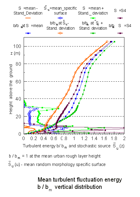
Based on this correlation, the equation for the mean turbulent fluctuation energy, b(z), for the URL layer is

and for the upper plain layer

where the mean eddy viscosity is given by

with being the turbulent scale function, following the Kolmogorov-Prandtl mixing length theory. The model presented above for the mean eddy viscosity is not the one obtained with the help of direct volume averaging procedures. It is based on the analysis references above and can be seen as an implicit result of averaged phenomena in the REV. The mean turbulent fluctuation energy is taken as an implicitly two-dimensional variable.

Closure schemes are required for the turbulent scale function and the drag resistance coefficient, . The result is a two-layer problem in the URL. Such a two-layer model was shown by Rodi et al. (1993) to be a way to treat near smooth wall turbulent transport modeling problems. The concept of a two-layer model near the wall surface was employed to better describe the turbulent characteristics close to the smooth wall below the nondimensional distance 80. In this sublayer a one-equation model was used for the turbulent kinetic energy k and a relationship like (24) for modeling the eddy viscosity close to the wall.

An equation for turbulent mass transfer, including the morphology functions, can be derived in the same way. In the UR layer as in the "porous" medium the equation for turbulent mass transfer in the urban atmosphere phase is (Travkin and Catton, 1994,1995,1998)

where is the turbulent local value of pollutant's mass fraction concentration in an air.

The morpho-convective dispersion type term (and

the morpho-diffusive term (and

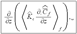
and the gradient of surficial mass transport term (and

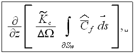
are very difficult to model - there are should be the morphology specific and exact simulations by using the samples of the medium.

The equation we simplified further to the equation often used in many applications suggesting somewhat partial inclusion of the phase exchange effect terms

where is the pollutant's gravitational precipitation modeling velocity, and the is the source term parameterizing the other morpho-transport terms in the VAT 2D upper scale urban pollutant's concentration equation.

The motion in the URL , equation

or

where the represents the all forms of flow resistance, we do not need to distinguish here the factor (1/2) as well.

In the plain layer

the turbulent kinetic energy equation in the porous UR layer

while in the plain layer this equation does not have the volumetric resistance term

where the mean eddy viscosity is given by

- the mass transport equation in fluid phase in the URL

- and in the plain layer

- and the mass transport equation in build-up phase

with

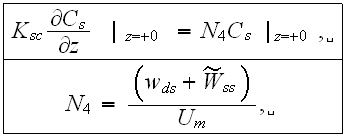
If 2-nd kind boundary conditions are chosen for the concentration fields, the boundary conditions for these equations are

where is the pollutant's capture constant at the ground - might be equal to zero, and the similar constant taken for the boundary in the buildings fraction of the medium,

the left boundary (at the entrance to URL)

3.7 Dimensionless Form of the Governing Equations - when

The scales have to be determined for all variables to make the governing equations dimensionless. The chosen scales are

with

The conservation equations in dimensionless form are (the different forms for rough and plain layer result from the assignment and for ) :

the equation of motion:

- for the URL when droping the (*) stars at the nondimension functions we get the nondimensional equation of momentum with the two parameters

- and for the ABL plain layer

the equation of turbulent fluctuation energy:

- for the URL

where is the porous medium turbulent kinetic energy coefficient exchange ratio

This equation would be having the appearance of

when the temperature gradient influence will be taken care of for the large horizontal dimension in the problem;

- and for the ABL plain layer

the mean turbulent eddy viscosity

the pollutant concentration equation for the air (street) phase

- for the URL: omitting the stars (*)

- and for the plain layer

where

the pollutant concentration equation for the build-up (solid) phase

with the bottom surface boundary condition:

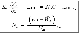
as soon as and if then at the ABL upper BC and at the

and the left side entrance Boundary Condition - taken for better analysis to be equal to a constant input value

Here we have only the 10 similarity numbers

and the number of functions to seek are 14

while the input functions and parameters are

How important the dimensionless analysis is one can find from numerous experimental works where the research done using the analogy of Homogeneous Mathematical Statements. For example, we can see in the typical paper by Nagabhushanaiah (1987) (just one among many of like approaches, also the old good review by Kalikov et al., 1986) where the drag resistance of the large building complexes were sought as via using the dimensionless complex in the formulae as the following one with the 5 parameters

which is the conventional thing for most experimental works. In this relation is the "boundary layer thickness above the bed within which there occurs velocity gradient zero at the bed to the maximum at the top", is the height of the building; is the projected width in the direction of the building; is the normal width of the building; is the pressure measured on the face of building at various tapings; is the free sreem velocity of wind approaching building in the wind tunnel above the boundary layer.

Obvious observation reading these experimental set-ups and data reduction methods is that the problem with the naturally physically seen two scales of phenomena in action - these problems being approached with the standard set of Homogeneous one scale fluid mechanics judgment.

Contrary to the Homogeneous medium treatment we used the two scale transport (and interests) concept and the results were capable to model the problem as the two scale one - even with the parametric inclusion of few effects. Many features are not available for the one scale -one phase simulation.

For example -

1) the inclusion of morphology properties directly into modeling equations is available and mandatory, even experimental features became available;

2) the modeling coefficients are directly tied to the physical and morphological properties of the task - in the specific URL's;

3) there are features of communications between the street air qualities and the buildings (second phase) air quality. More of that, even when the internal buildings pollutants sources introduced into the model, the level of concentration inside of the buildings can become much higher then of the street level. This experimentally found feature is not properly modeled when the only buildings air pollutant concentrations simulated as in a separate phase system;

4) the output model's data are presenting the values of some representative volume (REV) which is the final goal for the assessments of hazardous situation, otherwise the local concentration of pollutant's field should be volume averaged in some fashion and the concentration fluxes in that procedure will be simulated incorrectly if using the homogeneous GO theorem, etc.

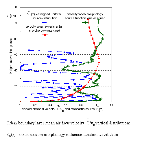
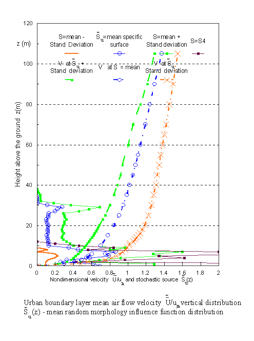
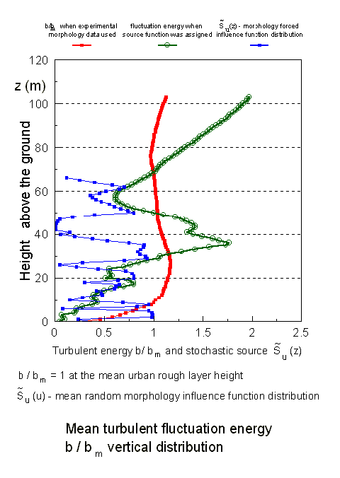
 How strong is the influence of additional morpho-induced terms in the VAT upper scale momentum equation on the velocity function is seen in this below figure:

Here is the picture of the boundary air velocity profiles based on calculations using one of the sets of morphological data,

It is seen, that the particular explicit statistical data on morphology of urban buildings and vegetation characterize to some extend the air velocity and the turbulent kinetic energy profiles in the URL (below).

 Few of the selected concentration profiles depend on parameters of the SVAT modeling equations

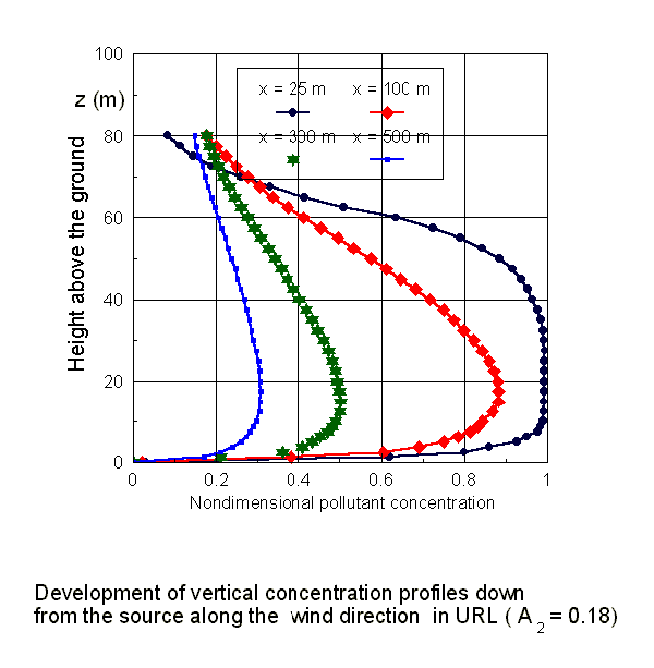
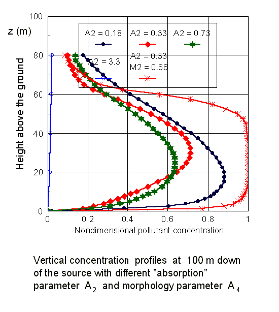
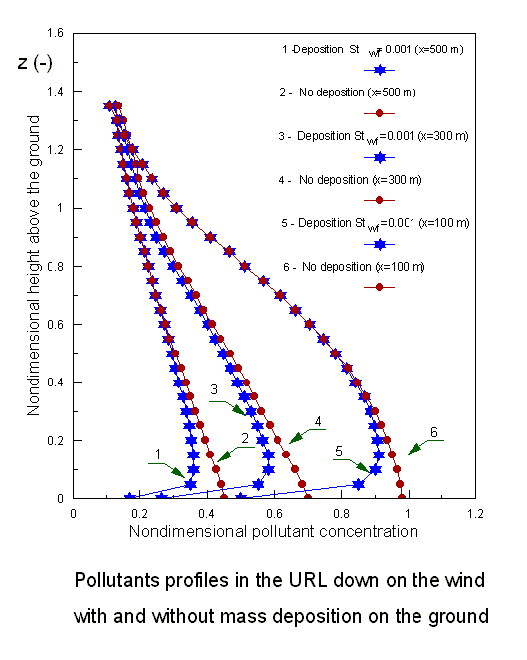
  Proceeding from the simulation results for the real urban morphology characteristics in one of local area in the city of Kiev we arrived to the conclusion that, specifically, the arrays of experimental data on the harmful impurity concentrations obtained in the lower part of the URL are significantly affected by the morphometric characteristics of the URL properties. That was obvious anyway. Still, it was apparent also that available models could not predict the increased levels (or absorbed due to influence of the second phase) of concentration of pollutants in the URL nor the atmospheric weather elements.

   Later in 1986-1989 the results and experience of scaled ABL modeling with incorporation of the region's surface industrial roughness morphology data were used in assessment of ABL pollution problems for the very large oil deposit exploration project “Tengiz” in Kazakhstan, which is now still under continuous development by international partners (including USA partners; Chevron).