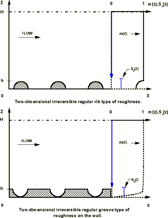
Fig. 1a Two-dimensional regular transformable (invertable groove type of roughness on the channel wall)
Turbulent flow and heat transfer over a surface with roughness on it has been shown treatable using porous media turbulent filtration theory - the VAT. This approach yields the basis for a unified description of an enormous spectrum of roughness layer morphologies as well as a scalable treatment of diverse engineering and scientific issues. When roughness' morphological properties are known as being assigned with spatial regularity that contributes to the simplification of the mathematical model as well as to closure modeling and numerical simulation. Some of the closures modeling elements were developed using experimental results. The results are then compared to theoretical and experimental studies of flow in channels with roughened walls and with smooth walls by allowing the roughness elements to become vanishingly small. The results of simulation of different roughness element morphologies demonstrate the interdependency of the roughness layer morphology, the mathematical formulation of the problem and the transport characteristics.
During years there has been a trend to create artificial types of roughness on surfaces to improve their effectiveness by varying some of the parameters describing them. The enhancement of heat transfer is sometimes achieved by using a porous insert or roughness on the channel walls, whereas in other cases the problem solution includes a complete filling of the channel with a porous media. Examples are found among heat exchangers, nuclear power stations, chemical process plants, and the relatively new area of porous radiant burners among others. Much of this work is based on a trial and error basis where judgement and past experience is used to suggest new directions in the search for improved surfaces.
The impact of a rough surface on transport phenomena is not a new subject. There have been many studies of the subject and, as a result, many correlations and theories found in the literature. When one tries to use these results, wide-ranging predictions of heat transfer and/or friction result. The primary reason for this is the lack of full accounting for the parameters that allow a particular surface to be mathematically represented by either correlation or theory.
To the contrary the VAT allows to apply a consistent approach to the problem, and a complete mathematical representation of roughened surfaces results.
We exhibit here few of the VAT based studied morphologies -
The first step is to outline initial equations from a set of turbulent transport equations. These equations are then made dimensionless by choosing an appropriate set of scales. Models for the turbulent mixing length, drag coefficients, and heat transfer coefficients are then developed to complete the model.
Many equations and features are the same or close in this problem and the Urban Rough Layer meteoelements and air pollution problem. The reason is that the same ground served for both fields. The VAT URL air pollution problem was firstly developed in the early 80-th, and then following those models the following one was created with few of students (the first was one with a very strong university courses background and active fellow from Germany H.Dichtl) while I continued VAT developments at UC Los Angeles, as for the widely different scales turbulent problem of transport in the porous or rough channels.
The averaging procedure starts with the lower scale (homogeneous) turbulent
transport equations (first set, for example, from Rodi, 1980 )
 The closure of these equations requires a turbulence model to evaluate the
Reynold-stress terms. A commonly used model is the
The closure of these equations requires a turbulence model to evaluate the
Reynold-stress terms. A commonly used model is the
![]()
 turbulence model. A version from Rodi (1980) is
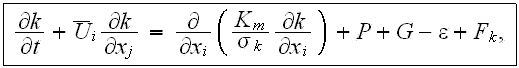

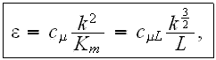
 is the buoyancy production (or destruction) term
Starting from this set of equations, different approaches are available for
computing flow over rough surfaces. Mathematical statements in most published
works describe the selected roughness elements in a way that depicts
morphology characteristics serving as external restricting parameters either
as boundary conditions or through the determination of a specific domain of
interest. In a number of experimental studies (Perry et al., 1969; Liou et
al., 1993, for example) and in a number of theoretical works (Tani, 1987;
Kader and Yaglom, 1984), the friction velocity
![]()
 and shear stress
![]()
 are assumed to be measured at the "wall" level. What this means, is that
![]()
 is actually assessed or measured somewhere in the bottom part of the
logarithmic velocity profile. This issue, not widely recognized, is the basis
for most rough surface investigations. The distance from the wall for a rough
surface is needed for each specific case of roughness morphology. For example,
in a tube, the friction velocity and wall shear stress are
is actually assessed or measured somewhere in the bottom part of the
logarithmic velocity profile. This issue, not widely recognized, is the basis
for most rough surface investigations. The distance from the wall for a rough
surface is needed for each specific case of roughness morphology. For example,
in a tube, the friction velocity and wall shear stress are
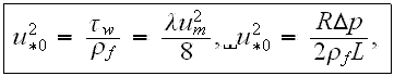
yielding the crucial quantity
![]()
 without real measurements near the wall.
The distance from the wall for which the shear stress concept has meaning
should be of interest. The uncertainty in the wall shear stress height
partially explains the appearance of additional terms in roughness surface
logarithmic velocity laws. Thus, Nikuradse's law of the a rough wall (2) for a
fully rough regime has an additive constant equal to
![]()
 when the dimensionless coordinate
![]()
 (70 or 80). Webb et al. (1971) dealt with this by using specific dependencies
for the roughness function
(70 or 80). Webb et al. (1971) dealt with this by using specific dependencies
for the roughness function
![]()
 .
The fact that in a fully rough regime, the drag resistance coefficient
.
The fact that in a fully rough regime, the drag resistance coefficient
![]()
 (friction factor) becomes independent of the friction velocity
![]()
 suggests that there should be correlations for each specific roughness
morphology and channel type.
suggests that there should be correlations for each specific roughness
morphology and channel type.
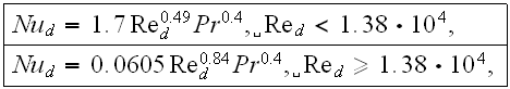
Youn et al. (1994) used numerical analysis to produce a correlation for the square rib roughness friction factor in a rectangular channel. Meanwhile, Liou et al. (1993) suggested a heat transfer coefficient correlation which reflects the impact of morphological parameters such as rib height and pitch on the average heat transfer for square ribbed roughness.
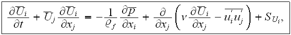
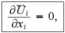
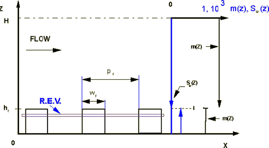
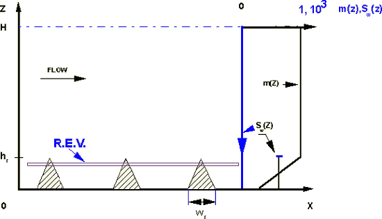
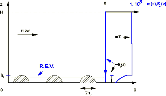
The present model was developed based on the assumption that the roughness elements are symmetrically shaped and regularly arranged. These assumptions greatly simplify the final mathematical statements and closure procedures. Some derivations for randomly arranged roughness elements were reported by Scherban et al. (1986a,b). The flow in the channel is assumed to be steady state, fully developed, turbulent and incompressible and the fluid properties are taken to be constant.
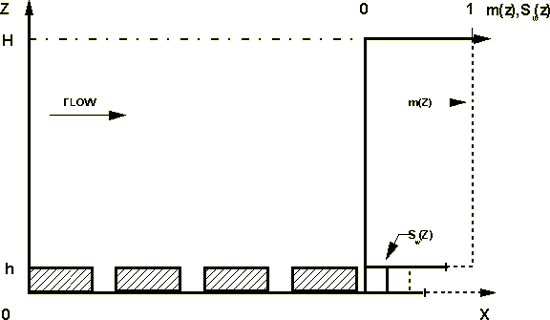
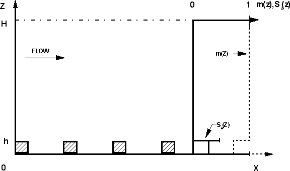
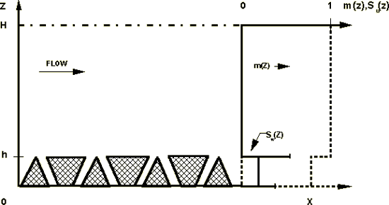
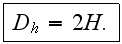
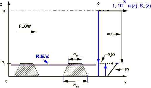
The channel investigated is two-dimensional (channel width is infinite) with both walls of the channel having the same roughness geometry, Fig. 7. To compare with results from the literature obtained with other channel types, the hydraulic diameter is defined by
Averaging the transport equations over the REV allows investigation of virtually an unlimited variety of morphology structures in a channel. The basic ideas of the averaging technique were developed for an atmospheric urban boundary layer by Scherban et al. (1986), Primak et al. (1986), Travkin and Catton (1992). With these ideas, a complex structures, composed of different morphology types, can be modeled (e.g. a channel with rough walls and a porous insert).
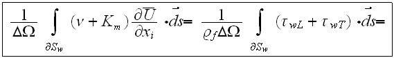
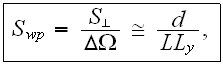
In this work the effect of highly rough walls on the flow and heat transfer in a two-dimensional symmetrical channel was investigated. The rough sublayer is treated as a heterogeneous porous medium. This method is based on averaging the transport equations in a REV, see Whitaker (1967, 1986a,b) for the laminar regime and Scherban et al.(1986a,b) for the turbulent regime. The horizontal dimensions of the REV are far greater than the characteristic dimensions of the roughness elements in the longitudinal direction and infinite in the transverse direction. In the case of regularly arranged roughness elements, the longitudinal dimension of one REV is typically one pitch of the roughness element (see Fig. 7).
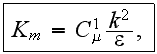
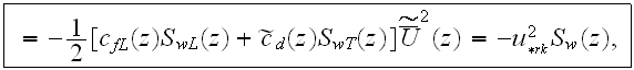
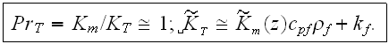
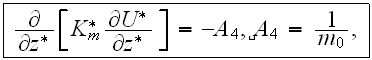
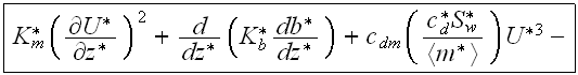
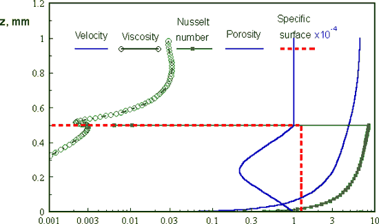
Independent treatment of turbulent energy transport in the fluid phase and energy transport in the solid phase, connected through the specific surface (the solid-fluid interface in the REV), allows more accurate modeling of the heat transfer mechanisms between the rough surface and the fluid phase. In the present transport model, the flow resistance of the rough wall is represented by a model with the second power of velocity and separate coefficients for each resistance mechanism (friction in the laminar zone, friction in the turbulent zone and form drag). For high Re numbers turbulent flow over rough walls the laminar friction drag can be neglected. The functions determining the morphology of the channel are the porosity
and the specific surface area
The porosity is the volume fraction open for the fluid phase in the REV while the specific surface area is the interface area of solid and fluid phase in the REV. A rough channel seen as to be divided into two layers:
- the rough layer
![]()
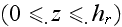 which has real heterogeneous characteristics, and
- the plain layer
which has real heterogeneous characteristics, and
- the plain layer
![]()
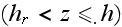 in core region of the channel which contains only the fluid phase.
These two layers can be artificially modeled by assigning appropriate values to the morphology functions.
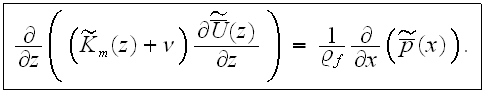
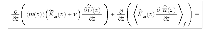
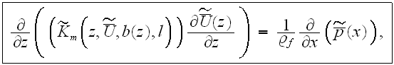
Taking into account the morphology structure in the rough layer, the
one-dimensional VAT equation for turbulent flow in the rough layer
![]()
 is, see Travkin and Catton (1994,1995,1998),
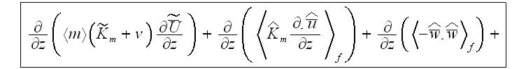
or neglecting the morpho-fluctuation terms
![]()
![]()
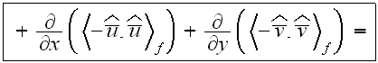
 and
and
![]()
 those demanding substantially larger effort for simulation (equations and
additional closure simulation) we would bring the following momentum equation
for modeling
those demanding substantially larger effort for simulation (equations and
additional closure simulation) we would bring the following momentum equation
for modeling

where
![]()
 is
the turbulent eddy viscosity, and the
is
the turbulent eddy viscosity, and the
![]()
 is the source term in this equation (meaning to serve as for inclusion of the
unknown level of influence of additional VAT terms).
is the source term in this equation (meaning to serve as for inclusion of the
unknown level of influence of additional VAT terms).
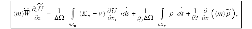
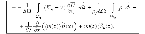
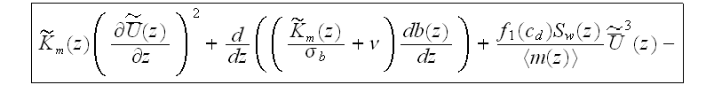
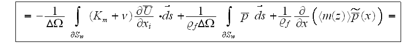
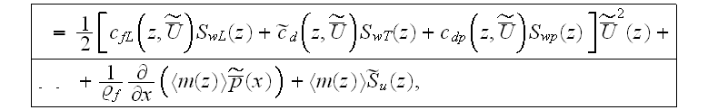
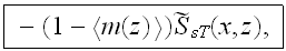
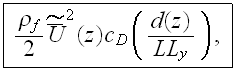
The last term on the left hand side of the equation for the rough layer and the two integral terms on the r.h.s. represent the flow resistance of the roughness elements. The diffusion-fluctuation term is on the l.h.s. The first term on the r.h.s. is the friction drag in the laminar and turbulent subareas regime of the obstacle surface, the second term is the form drag of the rough layer obstacles. It is interesting to note that the integro-differential equation accounting for a surface roughness was derived in a very different area of research dealing with nonlinear effects of transition in incompressible boundary layer theory (see Kachanov et al., 1993, Bogdanova-Ryzhova and Ryzhov, 1996).
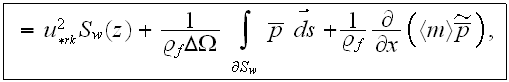
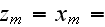
In the middle part of the channel
![]()
 ,
we have
,
we have
![]()
 and
and
![]()
 .
This simplifies equation (19) to
.
This simplifies equation (19) to
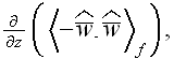
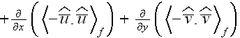
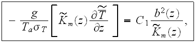
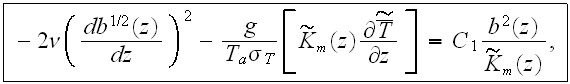
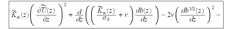
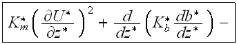
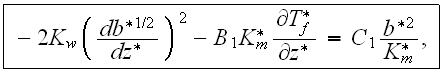
The volume drag resistance forces have to be taken into account in the turbulent fluctuation energy balance. Assuming that the loss of mean motion kinetic energy due to the pulsed character of the drag forces of the roughness elements is completely converted into turbulent fluctuation energy as done by Monin and Yaglom (1971) , and by Menzhulin (1970), the connecting correlation between drag forces and turbulent fluctuation energy for the rough layer is
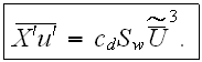
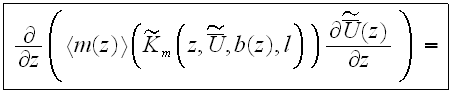
Based on this correlation, the equation for the mean turbulent fluctuation energy, b(z), for the rough layer is

and for the plain layer

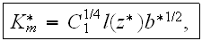
where the mean eddy viscosity is given by
with
![]()
 being the turbulent scale function, following the Kolmogorov-Prandtl mixing
length theory. The model presented above for the mean eddy viscosity is not
the one obtained with the help of direct volume averaging procedures. It is
based on the analysis references above and can be seen as an implicit result
of averaged phenomena in the REV. The mean turbulent fluctuation energy
being the turbulent scale function, following the Kolmogorov-Prandtl mixing
length theory. The model presented above for the mean eddy viscosity is not
the one obtained with the help of direct volume averaging procedures. It is
based on the analysis references above and can be seen as an implicit result
of averaged phenomena in the REV. The mean turbulent fluctuation energy
![]()
 is taken as an implicitly two-dimensional variable.
Closure schemes are required for the turbulent scale function
![]()
 and the drag resistance coefficient,
![]()
 .
The result is a two-layer problem. Such a two-layer model was shown by Rodi et
al. (1993) to be a way to treat near smooth wall turbulent transport modeling
problems. The concept of a two-layer model near the wall surface was employed
to better describe the turbulent characteristics close to the smooth wall
below the nondimensional distance
.
The result is a two-layer problem. Such a two-layer model was shown by Rodi et
al. (1993) to be a way to treat near smooth wall turbulent transport modeling
problems. The concept of a two-layer model near the wall surface was employed
to better describe the turbulent characteristics close to the smooth wall
below the nondimensional distance
![]()
 80. In this sublayer a one-equation model was used for the turbulent kinetic
energy k and a relationship like (24) for modeling the eddy viscosity close to
the wall.
80. In this sublayer a one-equation model was used for the turbulent kinetic
energy k and a relationship like (24) for modeling the eddy viscosity close to
the wall.
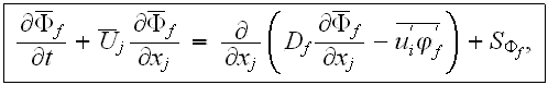
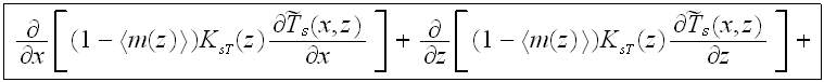
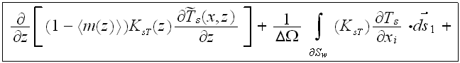
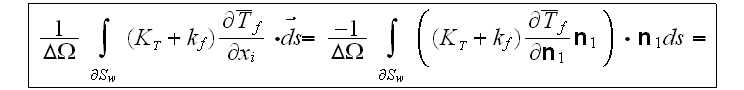
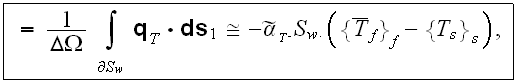
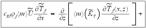
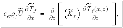
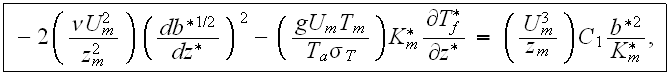
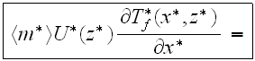
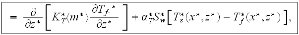
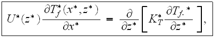
An equation for turbulent heat transfer, including the morphology functions, can be derived in the same way. In the rough layer as in the "porous" medium the equation for turbulent heat transfer in the fluid phase is (Travkin and Catton, 1994,1995,1998)
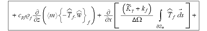
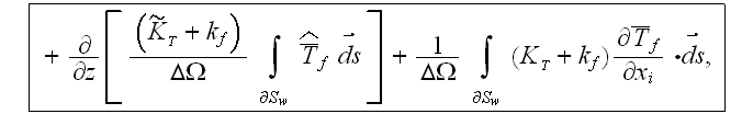
which we simplified further to the equation often used in the many applications suggesting somewhat partial inclusion of the phase exchange effect terms
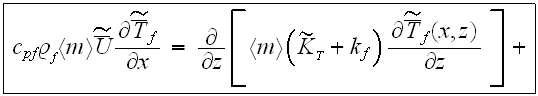
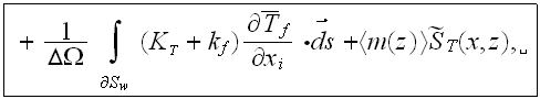
where the
![]()
 is the source term parameterizing the other terms in the VAT 2D upper scale
fluid temperature equation.
is the source term parameterizing the other terms in the VAT 2D upper scale
fluid temperature equation.
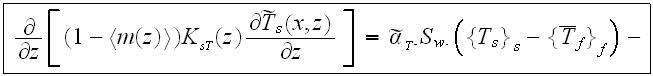
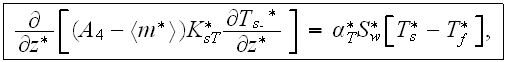
The solid phase upper scale averaged temperature equation can be derived in the form (we assume that the conductivity coefficient is not a constant value)
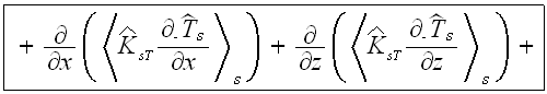
this equation after simplifications becomes
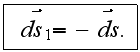
For the plain layer (as there is no heat transfer from solid to fluid in this domain), these two equations reduce to
The two-layer model, (19) - (28), is quite different from that seen in the literature, see for example work by Chen and Patel (1988) and by Arman and Rabas (1991, 1992). These workers use the expressions
in the near-wall region for the algebraic dependencies of eddy viscosity and dissipation rate and the turbulent kinetic energy equation uses the conventional production term given in (14). The problem is not treated as a two-layer problem and there is no relationship to the specific characteristics of the roughness elements.
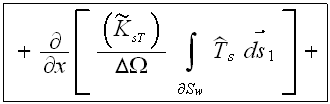
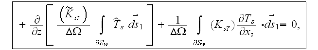
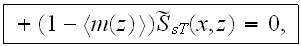
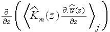
For closure of the integral terms in the rough layer equations, one has to integrate over the interface surface (between solid and fluid) in the REV. In the case of discrete obstacles on the wall, it is an integral over the obstacle surface.
![]()
 is
the square friction velocity at the upper boundary of surface roughness layer
is
the square friction velocity at the upper boundary of surface roughness layer
![]()
 averaged
over interface surface
averaged
over interface surface
![]()
 .
The closure of the morpho-diffusion term
.
The closure of the morpho-diffusion term
![]()
 we would set apart (include into the source tem) in the presented here
simplified VAT (SVAT) model. It's closure demands consideration and addition
of other tools those not presented in this model.
we would set apart (include into the source tem) in the presented here
simplified VAT (SVAT) model. It's closure demands consideration and addition
of other tools those not presented in this model.
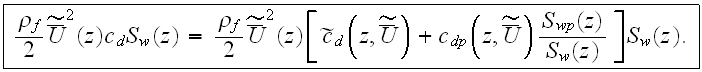
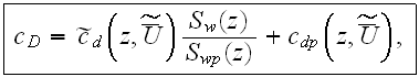
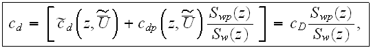
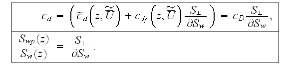
The closure scheme for the skin friction resistance terms in equation (19) is
with the general expressions, for example, for the laminar (if any exists) and turbulent part of the local boundary layer within the REV being
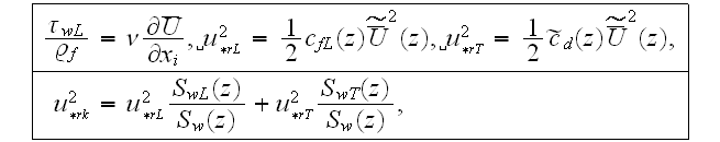
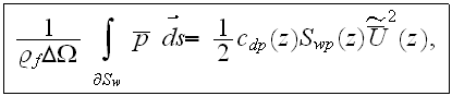
For turbulent flow over a rough wall, the laminar friction terms (index L) are usually negligible. The integral term for the drag resistance can be closed using the definition of the pressure resistance coefficient
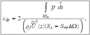
following the derivation of conventional drag resistance relationship
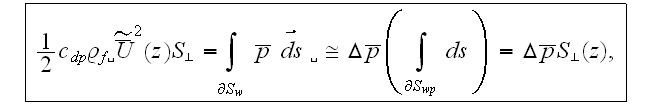
as soon as
with this coefficient, closure of the pressure integral term is
Closure of the heat exchange integral terms is based on the relationships
as soon as the heat exchange relation can be written as the conventional one
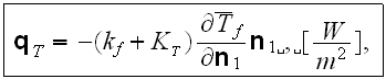
where
![]()
 is the outward directed from the solid phase normal vector. The final set of
equations includes the equations for turbulent fluctuation energy
(22) and (23), and the
correlation for the mean eddy viscosity (24).
These equations are
is the outward directed from the solid phase normal vector. The final set of
equations includes the equations for turbulent fluctuation energy
(22) and (23), and the
correlation for the mean eddy viscosity (24).
These equations are
- the equation of motion in the rough layer
![]()
 ,
,
- and in the plain layer
![]()

the turbulent kinetic energy equation in the porous wall layer

while in the plain layer this equation does not have the volumetric resistance term

where the mean eddy viscosity is given by

- the energy equation in fluid phase in the rough layer
- and in the plain layer
- and the energy equation in solid phase
with
The first term on the right-hand side of (34) is close in appearance to the
resistance term in the momentum equation of the discrete volume model
developed by Taylor and co-authors ( see, for example, Taylor et al., 1985;
Taylor and Hodge, 1993). The difference, however, results from the
incorporation of the local drag resistance coefficient
![]()
 and morphological factor
![]()
 for a plain channel (Taylor et al., 1985), or (d(y)R/(r Ly L) for a pipe model
(Taylor and Hodge, 1993), where
for a plain channel (Taylor et al., 1985), or (d(y)R/(r Ly L) for a pipe model
(Taylor and Hodge, 1993), where
![]()
 and
and
![]()
 are the spacing of the roughness elements on the wall in flow direction
![]()
 and perpendicular to the flow direction
![]()
 .
Meanwhile, in the reduced form of equation (34), the morphological factor
should be represented by the REV specific surface quantity
.
Meanwhile, in the reduced form of equation (34), the morphological factor
should be represented by the REV specific surface quantity
![]()
 and the resistance coefficient
![]()
 by the combined averaged over the interface surface friction and form
resistance coefficient.
by the combined averaged over the interface surface friction and form
resistance coefficient.
The blockage factors
![]()
 ,
,
![]()
 in the momentum equation derived by Taylor et al. (1985) can be viewed as
volume porosity functions that vary from the bottom of roughness element to
the top. Further development of the use of morphological factors for this
model are found in the work of James et al. (1993). To conclude, it can be
seen that the momentum and energy equations, eqs. (34,36), and ones in the discrete
element method by Taylor and co-authors are similar. Substantial differences
may be found when closure models are compared with the corresponding
coefficients.
in the momentum equation derived by Taylor et al. (1985) can be viewed as
volume porosity functions that vary from the bottom of roughness element to
the top. Further development of the use of morphological factors for this
model are found in the work of James et al. (1993). To conclude, it can be
seen that the momentum and energy equations, eqs. (34,36), and ones in the discrete
element method by Taylor and co-authors are similar. Substantial differences
may be found when closure models are compared with the corresponding
coefficients.
For closure of the above equations, the friction, drag and heat transfer coefficient functions are required. These coefficients have to be determined in accordance with the roughness geometry and the flow conditions. The pressure gradient term in equation (34) is modeled as a constant value over the channel.
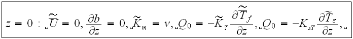
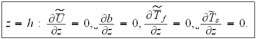
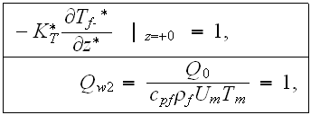
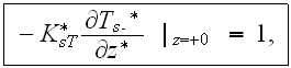
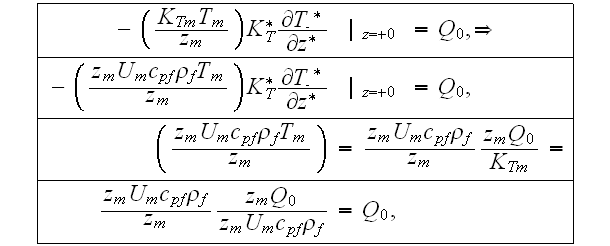
If 2-nd kind boundary conditions are chosen for the temperature fields, the boundary conditions for these equations are
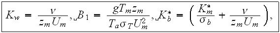
Scales have to be determined for all variables to make the governing equations dimensionless. The scales chosen are
 |
 |
 |
 |
 |
 |
 |
 |
 |
 |
 |
 |
 |
 |
 |
 |
 |
 |
 |
 |
Note that the characteristic length scale is different than the usual length
scale for rough channels (either channel diameter or roughness height). The
length scale used here is the ratio of the mean porosity to the mean specific
surface across the channel
![]()
 and represents the morphology characteristics of the channel. For a completely
smooth channel, this length scale is not appropriate
and represents the morphology characteristics of the channel. For a completely
smooth channel, this length scale is not appropriate
![]()
 .
The advantage is that the present model can easily be combined with other
morphology structures in the channel, e.g. porous media.
.
The advantage is that the present model can easily be combined with other
morphology structures in the channel, e.g. porous media.
The conservation equations in dimensionless form are (the different forms for
rough and plain layer result from the assignment
![]()
 and
and
![]()
 for
for
![]()
 )
:
)
:
the equation of motion:
- for the rough layer

- and for the plain layer
the equation of turbulent fluctuation energy:
- for the rough layer

which will be after deviding on
![]()


where
- and for the plain layer
the mean turbulent eddy viscosity
the energy equation for the fluid phase
- for the rough layer:
- and for the plain layer
where

the energy equation for the solid phase
with the bottom surface boundary condition:
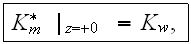
as soon as
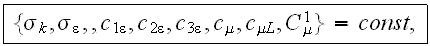
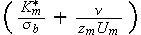
with the only 5 similarity numbers
 |
 |
 |
 |
 |
 |
 |
 |
 |

![$[-]$](/thermph/pic/vatrlstate__172.gif)
|
 |
 |
and the number of functions to seek are 10
 |
 |
 |
 |
 |
 |
 |
 |
 |
 |
 |
 |
 |
 |
 |
 |
 |
 |
 |
while the input functions and parameters are
 |
 |
 |
 |
 |
 |
 |
 |
 |
 |
 |
 |
 |
 |
 |
 |
here is again the function scales table
 |
 |
 |
 |
 |
 |
 |
 |
 |
 |
 |
 |
 |
 |
 |
 |
 |
 |
 |
 |
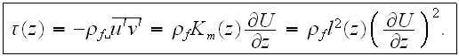
Turbulent mixing length theory is closely connected to the Reynolds-stress theory for turbulent flow. At a sufficient distance from the wall, the turbulent shear stress can be expressed with either the turbulent fluctuation velocities or the turbulent mixing length:
The profiles for different mixing length functions are shown in Fig.8.
Prandtl (1925) determined that a near wall mixing length is
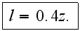
This correlation is a very general approximation to the mixing length
coefficient very close to the wall. As shown in Fig. 8(1) all common mixing
length approximations have a gradient of
![]()
 close to the wall. To make this simple and convenient approach suitable for
the core region of a duct (or the outer region of a boundary layer) the value
of
close to the wall. To make this simple and convenient approach suitable for
the core region of a duct (or the outer region of a boundary layer) the value
of
![]()
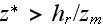
 is usually limited to the near wall region. Limits of
![]()
 (
(![]()
 radius of a pipe) and
![]()
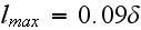 (
(![]()
 boundary layer thickness) are common (Taylor, Coleman and Hodge, 1992).
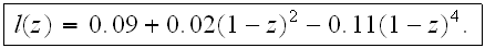
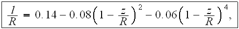
The abrupt discontinuity in the mixing length profile at the above limits was found to be unsuitable for the present numerical model (oscillations were caused). This led to using the following simple functional approximation for the mixing length:
Experiments carried out by Nikuradse (1932,1933) yielded results for the
turbulent mixing length both for a smooth and for rough pipes for
![]()
 .
For the mixing length he found the empirical relation
.
For the mixing length he found the empirical relation
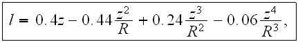
 values),
the higher order terms disappear and Prandtl's hypothesis is a good
approximation. The principal behavior in rectangular ducts can be assumed to
be similar to that of circular tubes. Numerical experiments using the Van
Driest damping factor on rough surfaces, where the wall shear stress is caused
almost entirely by the drag of the roughness elements and the effective
viscosity in the wall region, showed negligible effect on the flow.
values),
the higher order terms disappear and Prandtl's hypothesis is a good
approximation. The principal behavior in rectangular ducts can be assumed to
be similar to that of circular tubes. Numerical experiments using the Van
Driest damping factor on rough surfaces, where the wall shear stress is caused
almost entirely by the drag of the roughness elements and the effective
viscosity in the wall region, showed negligible effect on the flow.
These assumptions were confirmed with calculations for smooth and rough channels. For smooth channel calculations, without van Driest damping, the friction factor was up to three times higher than the calculated value from the Nikuradse correlation for smooth pipes. With damping, the friction factors show very good agreement with the Nikuradse equation, for both Prandtl and Nikuradse models. For walls with roughness elements, the damping factor has nearly no effect. For rectangular ribs of 10 mm height, the damping factor influenced the friction factor results less than 1%.
For many applications it is sufficient to know the increase in pressure drop in a channel or a pipe resulting from a roughened wall. The fluid resistance coefficient of a rough wall is often based on one reference velocity; either the maximum velocity or the mean velocity in the channel. However, it should be kept in mind that experimental friction factors are not appropriate for use in the present model because many other effects are needed to close the local resistence terms. Consequently, verification using the friction factor should be conducted carefully to account for all the effects that might influence the friction factor.
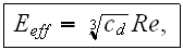
The drag coefficient for three-dimensional round-shaped obstacles was modeled
as a function of the local Reynolds number by Taylor et al. (1985). They
formulated a mean drag resistance coefficient,
![]()
 , model mainly as a function of the local element Reynolds number. The data
for numerically verifying the calculated drag resistance coefficient
, model mainly as a function of the local element Reynolds number. The data
for numerically verifying the calculated drag resistance coefficient
![]()
 and combined (approximately) coefficient
![]()
 for a rough channel morphology model were taken from Taylor et al. (1985),
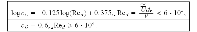
 is the diameter of a single projected roughness element on the channel wall
and includes information about the size and shape of a roughness element and
the local velocity. Taylor et al. corrected Schlichtings (1936) data, then
calibrated their model (1985). To apply this approach to the present model,
the volume resistance term of Taylor et al. (1985)
is the diameter of a single projected roughness element on the channel wall
and includes information about the size and shape of a roughness element and
the local velocity. Taylor et al. corrected Schlichtings (1936) data, then
calibrated their model (1985). To apply this approach to the present model,
the volume resistance term of Taylor et al. (1985)
(where
![]()
 is the spacing of the roughness elements in perpendicular to the flow
direction) is written in the notation of the present work using
is the spacing of the roughness elements in perpendicular to the flow
direction) is written in the notation of the present work using
so

while compared with the present model's turbulent resistance term
The final definition of the drag coefficient for the rough layer is then found using (56) and specifics of the rough layer following the dependencies
also the SVAT simplified bulk resistance coefficient is
and finaly these coefficients can be mutually evaluated via
It can clearly be seen from this comparison that the friction drag of the obstacle surface, in the expression for the volume resistance (58), has been taken into account in the resulting dependency. This approach seems reasonable for turbulent flow despite the fact that the friction drag is apparently a negligible part of the total drag in this situation. Furthermore, calibration of the drag resistance model with experimental values of different workers was required for possibly simple model.
To provide a tool for comparing the performance of different roughness geometries it is necessary to have a numerical model of the drag resistance of a single roughness element. Approximations of the roughness parameter (i.e. friction factor) for regular arrangements of rectangular ribs have been made by Dalle Donne and Meyer (1977), Baumann (1978) and Meyer (1979). These approximations are based on a database of experimental results, yet no model existed at the time which included information about the shape of the ribs.
To develop a model for the local drag resistance of a single rib in a regular
arrangement of ribs, important parameters that are likely to influence the
drag are considered: the shape of the ribs, the flow conditions (i.e. the
![]()
 number) and the arrangement of the ribs (ratio of height to pitch).
For highly rough walls, the boundary layer mechanisms important for evaluation
of smooth walls are no longer valid. The (longitudinally averaged) wall
friction is almost entirely due to the drag of the set of obstacles. Therefore
the friction of a highly rough wall seems to be caused more by the swerling
flow around an aggregate of bodies with respect to their mutual position in an
arrangement of similar obstacles around and that they are wall-mounted than by
viscous forces in the laminar sublayer. The results of experiments conducted
with single obstacles in the free-stream flow are not applicable because of
the influence of the position of adjacent obstacles, up- and downstream, and
the velocity boundary condition at the wall
(![]()
 ).
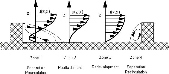
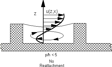
Flow reattachment and redevelopment (Fig. 9) between the obstacles is assumed
for ratios of pitch to height of more than 4-6. With redeveloped flow
(positive local fluid velocity over the whole channel crossection, see Fig.
9), the mechanisms of single obstacle form drag (fluid deflection, separation
and reattachment) can be used as an approximation.
).
Flow reattachment and redevelopment (Fig. 9) between the obstacles is assumed
for ratios of pitch to height of more than 4-6. With redeveloped flow
(positive local fluid velocity over the whole channel crossection, see Fig.
9), the mechanisms of single obstacle form drag (fluid deflection, separation
and reattachment) can be used as an approximation.
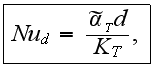
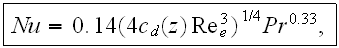
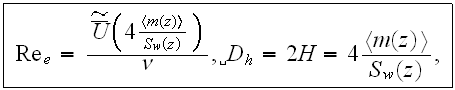
To close the energy equations, a heat transfer coefficient, αT, has to be found. The mechanism of heat transfer in turbulent flow is closely connected to the phenomenon of momentum transfer. In the literature one can find a great deal on heat transfer from smooth and rough walls. But, as most of the values are averaged over the rough layer, it is difficult to find data for local heat transfer. A correlation found for the local heat transfer coefficient for three-dimensional round-shaped obstacles is that of Taylor et al. (1989) and Chakroun and Taylor (1992),
where the local Nu-number is defined as
with the local obstacle diameter
![]()
 To show that the local Nu-number averaged over the REV can be applied to the
present model, we separate the term for heat transfer from a solid element to
the fluid from the energy equation used by Chakroun and Taylor (1992),
To show that the local Nu-number averaged over the REV can be applied to the
present model, we separate the term for heat transfer from a solid element to
the fluid from the energy equation used by Chakroun and Taylor (1992),
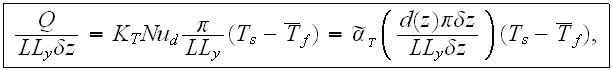
where
![]()
 denotes the height of the control volume. The equivalent term in the energy
equation of the present model is
denotes the height of the control volume. The equivalent term in the energy
equation of the present model is
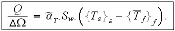
Using the notation of the present model, we can relate terms in equation (62) to those in equation (63)
Dichtl (1992) showed that the transfer term developed by Chakroun and Taylor (1992) and the present model are congruent. These relations were designed for three-dimensional round-shaped obstacles. It is not applicable to two-dimensional ribs because the length scale used in the Reynolds-number is inappropriate.
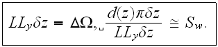
The Chakroun and Taylor (1992) model was compared with a correlation of Kharitonov et al. (1987) which was originally for heat transfer in a porous media consisting of spheres
where
(see Travkin and Catton, 1992,1995; Gratton et al., 1996). The length scale in Re e is (if applied to two-dimensional obstacles) proportional to the distance between the ribs,
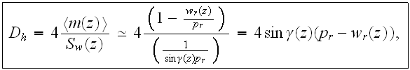
where
![]()
 is the local incline of the rib surface and wr(z) is the local width of the
rib and is the "hydraulic" diameter (Dichtl, 1992). Further development of
heat transfer models for ribs could be based on this method because it
includes the characteristics important for two-dimensional obstacles.
is the local incline of the rib surface and wr(z) is the local width of the
rib and is the "hydraulic" diameter (Dichtl, 1992). Further development of
heat transfer models for ribs could be based on this method because it
includes the characteristics important for two-dimensional obstacles.
It is apparent that there are different ways to treat a channel with a change
in the morphology structure: is a channel with (considerable high) roughness
elements on the wall an open channel with obstacles in it or a porous channel
with an open part? There is no general answer to this question, though the
more universal way seems to be to treat the entire channel as if it were
heterogeneous medium and form an open part of the channel by assigning the
morphology functions
![]()
 and
and
![]()
 in the plain layer
![]()
 to 1 and 0, respectively. This allows the treatment of complex morphologies
and even porous media with the same model (Travkin and Catton, 1992).
to 1 and 0, respectively. This allows the treatment of complex morphologies
and even porous media with the same model (Travkin and Catton, 1992).
Most studies of rough surface flow are based either on the assumption that a rough wall can be treated as a smooth wall with higher friction or consider roughness elements as wall deformations and compute the flow two-dimensionally along the surface.
To determine how well the transport model and the turbulence coefficients (in particular the turbulent mixing length correlations) represent the physical process, velocity profiles and friction factors for channels with smooth walls were calculated and compared to well-accepted correlations.
One can see the different regimes of turbulent flow from the calculated
velocity profile for a smooth wall (Fig.10). Below
z+ = 10, in the laminar sublayer, the velocity increase
![]()
 is linear. In the core region
![]()
 ,
the velocity profile is logarithmic, while for
,
the velocity profile is logarithmic, while for
![]()
 there is a transitional region between the laminar and the fully turbulent
layer. The theoretical profiles for the laminar and for the turbulent region
there is a transitional region between the laminar and the fully turbulent
layer. The theoretical profiles for the laminar and for the turbulent region
laminar -
![]()

![]()
and turbulent
![]()
are presented in Fig. 10. The computed profile shows good agreement with the analytical model in both regions. Flow through a smooth channel was calculated for different pressure gradients and channel dimensions, resulting in different Reynolds-numbers. The calculated friction factors were compared to common approximations; the Blasius formula
and the Nikuradse correlation
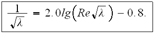
Fig. 11 shows excellent agreement between the computed friction factors (based on both mixing length models given above and the correlations formulae). The maximum deviations are less than 10% for both Prandtl and Nikuradse mixing length models with a better comparison with the Nikuradse model at the higher Reynolds numbers and with the Prandtl model at the lower Reynolds numbers. All in all, the difference between both models is small, so both models represent the turbulent intensity in the channel quite well. The Nikuradse mixing length model (Model B ) was chosen because of the expected higher turbulence intensity in a rough channel.
Better characterizing the more complicated morphology of a porous media leads to increasing the number of parameters while improving the methods and models of interconnection among the new parameters. Questions arise primarily in the area of closure modeling, independent of one's choice of governing equations. Using a very simple mathematical model of a biporous medium, Fong and Mulkey (1989) showed the great influence of more accurately examining the morphological structure of the medium. They use different diffusion equation for each medium, coarse and fine. However, the only features of the medium morphology taken into account were the two types of structures. The diffusion equation used in the fine structure was particularly simple, yet yielded a significant improvement.
The consequence of averaging the morphology structure over a Representative Elementary Volume (REV) is that one can look at the medium in the channel in two different ways:
- fluid and solid separated as physical fields;
- fluid and solid "homogenized" each in its volumetric subdomain.
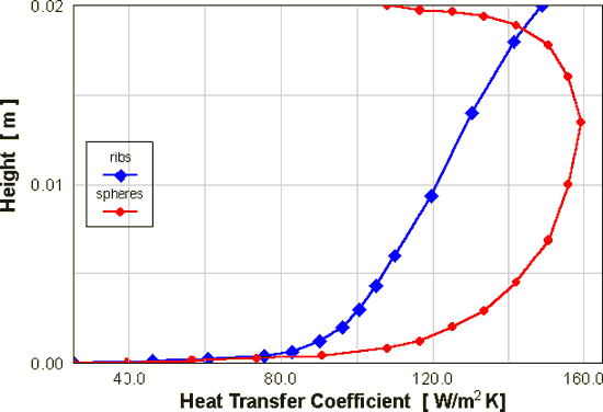
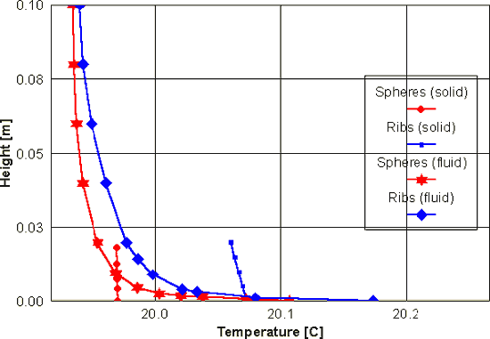
The two characteristic roughness elements are chosen to compare the results
for the same input channel conditions: a) 2D rectangular ribs; and b)
3D spheres. The height of the elements was 0.02 m with a rectangular
cross-section width of 0.04 m, and a channel half-width of 0.1 m; the pitch
for the two-dimensional roughness elements is 0.2 m while for the
three-dimensional obstacles it is 0.1 m. The calculations were done using a
two-temperature model flow of air with an inlet pressure gradient of -100
![]()
![$[N/m^{2}]$](/thermph/pic/vatrlstate__282.gif) ,
an inlet temperature of 20
,
an inlet temperature of 20
![]()
![$[C^{\circ }]$](/thermph/pic/vatrlstate__283.gif) ,
and a constant heat flux on the wall of 20
,
and a constant heat flux on the wall of 20
![]()
![$[W/m^{2}]$](/thermph/pic/vatrlstate__284.gif) .
.
The flow resistance of a rough wall is caused by different effects, though the dominant mechanism in a turbulent regime is the form drag of roughness elements. When one compares results from a rough two-dimensional plain channel (investigated in this work) with results of a rough pipe, another scaling problem arises. If the roughness elements reach a considerable height (compared to the channel dimensions), the effect of the blockage ratio (maximal to minimal area open to flow) is not the same in the flat channel and the pipe. This problem was not treated in the present work. To compare the present results with experimental results in pipes, the same roughness height as in the tube was taken to obtain the same wall shear stress.
The ratio of a pitch to height, as known, is a very important parameter for
regular morphology roughness. For
![]()
 of 5 or less, the deviations from experimental data were unacceptable high.
This indicates that the drag of a single rib is reduced due to the wake region
of the upstream rib. Therefore a factor, which represents the shading of ribs,
has to be included in the present drag resistance model. As the effect of the
shading must be evaluated locally for the present model, various aspects have
to be considered:
of 5 or less, the deviations from experimental data were unacceptable high.
This indicates that the drag of a single rib is reduced due to the wake region
of the upstream rib. Therefore a factor, which represents the shading of ribs,
has to be included in the present drag resistance model. As the effect of the
shading must be evaluated locally for the present model, various aspects have
to be considered:
- the influence of rib height to pitch,
- the influence of the rib shape,
- the influence of the Reynold-number on the wake formation for different rib shapes.
Lewis (1975) and by Kader (1977) considered this. They look at the wake behind the ribs as if it were solid (no flow in it). If the next rib is located in the wake region, the part which is affected by the simplified wake region causes no drag. The local drag coefficient developed by Taylor et al. (1985) for round-shaped three-dimensional obstacles has the same limits. Taylor et al. propose to shift the effective wall location for dense arrays of roughness elements and thus neglect the flow in the shaded layer.
For further improvement of the drag resistance model for two-dimensional ribs some other properties of the rib shape should be included in the model. At this time, only the local fluid deflection is used as a criterion for including the influence of Re-number on the drag coefficient. Consequently, sharp edges (like the top of a triangular rib) do not affect the local drag coefficient in the present model. In reality the flow separates at sharp edges and there is no pressure recovery at the backside of the rib, whereas the point of the flow separation is likely to vary with the Reynolds number for a smooth top (e.g. semi-circular rib).
The velocity, mean kinetic energy and turbulent viscosity profiles given in Figs. 12-14 achieve what would be expected for this kind of comparison. However, the temperature profiles show no such a good agreement, see Figs. 14-16. The results and comparison of application of different closure coefficients will be given later.
To verify the results of drag resistance model computations for rectangular
rib roughness, comparisons were made with the experimental data of Webb et al.
(1971). In his experiments, a pipe with an inner diameter of 36.83mm fitted
with transverse rectangular ribs was used. The rib heights varied from 0.036mm
to 1.47mm, i.e.
![]()
 ratios varied from 0.01 to 0.04. The agreement of the computed results with
the experimental data is generally good, with a maximum deviation of 15% (see
Fig. 17).
ratios varied from 0.01 to 0.04. The agreement of the computed results with
the experimental data is generally good, with a maximum deviation of 15% (see
Fig. 17).
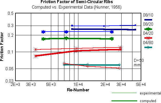
The experimental data generated by Nunner (1956) was used as a benchmark for the computed friction factors for a surface roughened with semi-circular ribs, see (Fig. 17). Nunner used a pipe with a 50mm inner diameter and semi-circular ribs with a radius of 2mm and of 4mm. The pitch to height ratio varied from 2 (what is in this case the densest arrangement) to 80.
The results shown in Fig. 17 indicate good
agreement for
![]()
 ,
while the lower
,
while the lower
![]()
 -ratios showed the limits of the drag resistance model used in this work. It
does not consider the wake of the upstream rib. For
-ratios showed the limits of the drag resistance model used in this work. It
does not consider the wake of the upstream rib. For
![]()
 the predicted friction factor was 40% higher than the experimental value and
for
the predicted friction factor was 40% higher than the experimental value and
for
![]()
 the deviation was 500%. To understand this large deviation, one has to look at
the trends of the experimental and computed values as the
the deviation was 500%. To understand this large deviation, one has to look at
the trends of the experimental and computed values as the
![]()
 ratio is decreased (the friction factors are averaged values in the turbulent
regime):
ratio is decreased (the friction factors are averaged values in the turbulent
regime):
![]()
 20
10
5
2
20
10
5
2
experimental
![]()
 0.23
0.31
0.25
0.08
0.23
0.31
0.25
0.08
computed
![]()
 0.19
0.27
0.34
0.45
0.19
0.27
0.34
0.45
In contrast to the experimental friction factors, the computed friction
factors rise for decreasing
![]()
 .
The drag resistance model of Taylor et al. (1985) has the same problem (see
the next section) for small
.
The drag resistance model of Taylor et al. (1985) has the same problem (see
the next section) for small
![]()
 ratios. They solved this problem with a variable (virtual) wall location.
Not enough reliable data for other geometries (trapezoidal and triangular ribs) could be found to verify the numerical results. It can be assumed, however, that by extrapolating the results from semicircular and rectangular ribs one might obtain reasonable predictions of the flow resistance for these geometries.
To compute the local drag resistance, a model developed by Taylor et al.
(1985) was used that was, according to the authors, verified for all
geometries (spheres, half-spheres, cones, cylinders) investigated in this
work. The model has not been tested extensively in this work. The experiments
of Schlichting (1936), however, were recalculated to test the implementation
of the drag resistance model. The results showed generally good agreement for
![]()
 ratios greater than 5, while for smaller
![]()
 deviations from experimental values increased. For dense packed spheres the
deviation reached 1000%. Taylor et al. recommend an artificial wall location
of 0.2 sphere diameters below the crest of the spheres for this case to
account for the almost total flow blockage below this plane.
deviations from experimental values increased. For dense packed spheres the
deviation reached 1000%. Taylor et al. recommend an artificial wall location
of 0.2 sphere diameters below the crest of the spheres for this case to
account for the almost total flow blockage below this plane.
In this work two models for the local heat transfer coefficient are used. The Taylor et al. (1989) and Chakroun and Taylor (1992) models were calibrated for three-dimensional round-shaped roughness elements and boundary layer flow. The Kharitonov, Plakseev et al. (Kokorev et al., 1987) model was originally designed for a porous medium consisting of spherical elements.
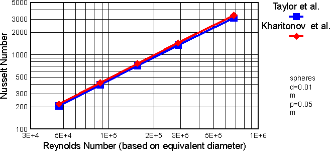
Both models give virtually identical predictions for the heat transfer for a
surface fitted with spheres. In Fig. 18 one can
see that the difference between the two models is less than 6% for a
![]()
 and less than 9% for
![]()
 (diameter of spheres 10mm, height of the flat channel 100mm).
The above heat transfer models could be compared using a surface roughened
with three-dimensional round-shaped obstacles. The results for both models are
nearly identical for spheres ( see Fig. 18)
whereas for the other geometries (half-spheres, cylinders and cones), the
Kharitonov model generally yields a 50% lower Nusselt number than the Taylor
et al. model. The calculated differences in the values of the local heat
transfer coefficient,
![]()
 are significant (Fig.19).
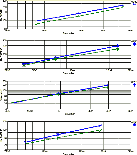
A comparison of the channel Nusselt numbers for different geometries can be seen in Fig. 18. It is noteworthy that the Kharitonov's et al. model yields the Nusselt number of a surface with two-dimensional semi-circular ribs. Comparison with the data of Nunner (1956) showed good agreement for ratios of pitch to height between 10 and 20 (deviation less than 25%) and reasonable agreement for a larger and smaller pitch to height ratios (deviation less than 50%). The prediction for rectangular ribs is not very good; deviations of 100-200% from the experimental data of Nunner were obtained.
For other three-dimensional geometries (half-spheres, cones, cylinders) the model of Kharitonov, Plakseev et al. generally predicts 30-50% lower Nusselt-numbers than the model of Chakroun and Taylor (1992).
Predictions of heat transfer for two-dimensional obstacles were also made with these heat transfer models. For two-dimensional half-circular ribs, the model of Kharitonov yielded reasonable results, with a deviation of less than 30% from the Nusselt numbers measured by Nunner, 1956 (Fig. 20). For rectangular ribs, the predictions were more than 100% too high, most likely because Kharitonov et al. developed the model for globular (with smooth shape) porous medium heat transfer phenomena.
The model of Taylor et al. (1989) predicts Nusselt number values for a channel with two-dimensional roughnesses that are far too high.
A common engineering problem is the optimization of heat transfer. If rough surfaces are used, the enhanced heat transfer is accompanied by an increased pressure drop. An extensive literature exists on the issue of enhanced heat transfer optimization. Different roughness elements morphologies attract attention because they show potential for heat transfer optimization. Among the latest effort is a study by Tiggelbeck et al. (1991) where the roughness enhancement was angled delta winglets intended to increase vortex generation on the gas side of compact heat exchangers. Lau et al. (1991) compared the thermal performance of angled rows of full and discrete ribs.
The current modeling approach allows the experimental data to be presented in a consistent manner along with morphology of the roughness elements. This issue seems to be a great obstacle when researchers in different fields explain their experimental data, see, for example, Taslim and Spring (1994), or Shaukatullah and Gaynes (1995). In other studies, where correlations were obtained from the experimental data, the lack of a general morphological description makes it almost impossible to use the correlation for a surface with even insignificantly different roughness morphology (Jubran et al., 1993).
A few results of rough surface heat transfer efficiency, the ratio of heat transfer to pumping power, were obtained. To express the results, the efficiency model as defined by Hijikata and Mori (1987),
was used in the analysis as a measure of the surface efficiency. In Fig. 21, the efficiency of a channel fitted with semicircular ribs is shown. The hydraulic diameter was taken to be 50mm, the rib pitch to be 41mm and the rib height varied from 1mm to 6mm.
The results indicate that the best performance was found for the highest ribs (enhancement ratio more than 1.8) while the smallest ribs resulted in a lower efficiency than a smooth channel. For higher pumping power, the enhancement ratio is lower and nearly the same for all rib heights. The lower enhancement rate is mainly due to the decreasing friction factor of a smooth wall at higher Reynolds number while the friction factor for rough walls is approximately constant.
The later modeling of the two scale semiconductor's heat coolers data have casted more insight on this crucial importancy issue. Analysis of known methods for determination of effective transport parameters and criteria were developed for the thermal effectiveness of a heterogeneous heat transfer device or medium later in 90th and were published in -Travkin and Catton, 2001; Travkin et al., 1998; Travkin et al., 2001a; Travkin 2001. These criteria are not the same as ones used for homogeneous devices and processes and consequently have the features of heterogeneous transport explicitly included as the medium morphology characteristics, for example.
The first step was to study fundamental problems of heat enhancing surfaces (2D-3D heat sinks).
The scaled VAT formulation allows one to include and highlight phenomena that are not observable when conventional homogeneous modeling is used-
Flow between ribs with different pitch to height ratios
Comparison of Nusselt Numbers Calculated from Heat Transfer. Models of Taylor et al. Kharitonov et al. (all dimensionless values based on the pipe-equivalent diameter of the flat channel D=0.4 m)
Arman, B., and Rabas, T.J., 1991. Prediction of the Pressure Drop in Transverse, Repeated Rib Tubes with Numerical Modeling, Proceedings of Fouling and Enhancement Interactions Conference, ASME HTD Vol.164, pp. 93 99.
Arman, B., and Rabas, T.J., 1992. Disruption Shape Effects on the Performance of Enhanced Tubes with the Separation and Reattachment Mechanism, Proceedings of 28th National Heat Transfer Conference, ASME HTD Vol. 202, pp.67 75.
Baumann, W., 1978. Geschwindigkeitsverteilung bei turbulenter Stroemung an rauhen Waenden, Kernforschungszentrum Karlsruhe, KfK Berichte 2618 and 2680.
Baumann, W., Rehme K., 1975. Friction correlations for rectangular roughnesses, Int. J. Heat Mass Transfer, Vol.18, pp.1189 1197.
Bogdanova-Ryzhova, E.V. and Ryzhov, O.S., 1996. Forced Nonlinear Disturbances in Incompressible Boundary Layers, Phys. Fluids, Vol. 8, No. 1, pp. 163 - 174.
Chakroun, W.,Taylor R.P., 1992. The effects of modestly strong acceleration on heat transfer in the turbulent rough wall boundary layer, ASME HTD Vol. 202, pp.57 66.
Chen, H.C. and Patel, V.C., 1988. Near-Wall Turbulence Models for Complex Flows Including Separation, AIAA Journal, Vol. 26, No. 6, pp. 641-648.
Coleman, H.W., Hodge B.K., and Taylor R.P., 1984. A re evaluation of Schlichting's surface roughness experiment, Journal of Fluids Engineering, Vol. 106, pp.60 65.
Dalle Donne, M.,Meyer L., 1977. Turbulent convective heat transfer from rough surfaces with two dimensional rectangular ribs, Int. J. Heat and Mass Transfer, Vol.20, pp.583 620.
Dichtl, H., 1992. Flow and Heat Transfer in Channels with Rough Walls, Diploma Thesis (for the Technical University of Munich), The University of California, Los Angeles, 100 pgs.
Dubov, A.S., Bykova, L.P., and Marunich, S.V., 1978. Turbulence in Phytocenosis, Gidrometeoizdat, Leningrad, p. 183.
Durgin, F. H., Chock, A. W., 1982. Pedestrian Level Winds: A Brief Review, Journal of the Structural Division, American Society of Civil Engineers, Vol. 108, No. 8, pp. 1751-1767.
Fong, F. K. and Mulkey, L. E., 1989. Simulation of Solute Transport in Aggregated Media, AIChE Journal, Vol. 35, No. 4, pp. 670 672.
Ganesh, R.K., 1994. The Minimum Drag Profile in Laminar Flow: A Numerical Way, Journal of Fluids Engineering, Vol. 116, No. 3, pp. 456-462.
Gratton, L., Travkin, V.S., and Catton, I., 1993. Transport Coefficient Dependence upon Solid Phase Morphology for Single Phase Convective Transport in Porous Media, Heat Transfer in Porous Media, ASME HTD-Vol. 240, pp. 11-21.
Hijikata, K.,Mori Y., 1987. Fundamental study of heat transfer augmentation of tube inside surface by cascade smooth surface promoters, Waerme und Stoffuebertragung, Vol.21, pp.115 124.
James, C.A., Hodge, B.K., and Taylor, R.P., 1993. A Discrete Element Method for the Prediction of Friction and Heat Transfer Characteristics of Fully-Developed Turbulent Flow in Tubes with Rib Roughness, Turbulent Enhanced Heat Transfer, ASME HTD-Vol. 239, pp. 9-18.
Jubran, B.A., Hamdan, M.A., and Abdualh, R.M., 1993. Enhanced Heat Transfer, Missing Pin, and Optimization for Cylindrical Pin Fin Arrays, J. Heat Transfer, Vol. 115, No. 3, pp. 576 - 583.
Kachanov, Y.S., Ryzhov, O.S., and Smith, F.T., 1993. Formation of Solitons in Transitional Boundary Layers: Theory and Experiment, J. Fluid Mech., Vol. 191, pp. 273 - ??
Kader, B.A., 1977. Hydraulic resistance of surfaces covered with two dimensional roughness with large Reynolds numbers, Teoreticheskie Osnovy Khimicheskoi Tekhnologii, Vol.11, No.3, pp.393 404, (in Russian).
Kader, B.A.,Yaglom A.M., 1977. Turbulent heat and mass transfer from a wall with parallel roughness ridges, Int. J. Heat and Mass Transfer, Vol. 20, pp.345 357.
Kader, B. A. and Yaglom, A. M., 1984. Effect of Roughness and Longitudinal Pressure Gradient on Turbulent Boundary Layers, in Itogi Nauki I Tekhniki. Mekhanika Zhidkosti I Gasa, Vol. 18, pp. 3-111.
Kalikov, V. N., Nekrasov, I.V., Ordanovich, A.E., and Khudyakov, G.E., 1986. Simulation of Wind Interaction with Different Engineering and Natural Objects in Wind Tunnels, in Itogi Nauki I Tekhniki. Mekhanika Zhidkosti I Gasa, Vol. 20, pp. 140-205.
Kokorev V.I., Subbotin V.N., Fedoseev V.N., 1987. Intercommunication of hydraulic resistance and heat transfer in porous media, Teplofiz. Vys. Temp., Vol. 25, No.1, pp.92-97, (in Russian).
Lau, S.C., McMillin, R.D., and Han, J.C., 1991. Heat Transfer Characteristics of Turbulent Flow in a Square Channel with Angled Discrete Ribs, J. Turbomachinery, Vol. 113, No.3, pp. 367-374.
Lewis, M.J., 1975. An elementary analysis for predicting the momentum and heat transfer characteristics of a hydraulically rough surface, Journal of Heat Transfer, Vol. 97, pp.249 254.
Liou, T.-M., Hwang, J.-J., and Chen, S.-H., 1993. Simulation and Measurement of Enhanced Turbulent Heat Transfer in a Channel with Periodic Ribs on One Principal Wall, Int. J. Heat Mass Transfer, Vol. 36, No. 2, pp. 507-517.
Menzhulin, G. V., 1970. On Methodic of Meteorology Regime Calculation in Plant Community, Meteorology and Hydrology, No. 2, pp. 92-99.
Meyer, L., 1979. Turbulente Stroemung an Einzel und Mehrfachrauhigkeiten im Plattenkanal, Kernforschungszentrum Karlsruhe, KfK Bericht 2764.
Monin, A.S. and Yaglom, A.M., Statistical Fluid Mechanics, MIT Press, Cambridge, MA, 1971.
Nikuradse, J., 1932. Gesetzmaessigkeit der turbulenten Stroemung in glatten Rohren, VDI Forschungsheft, No.356.
Nikuradse, J., 1933. Stroemungsgesetze in rauhen Rohren, VDI Forschungsheft, No.361.
Nunner, W., 1956. Wärmeübergang und Druckabfall in rauhen Rohren, VDI - Forschungsheft, No.455.
Perry, A. E., Schofield, W. H., and Joubert, P. N., 1969. Rough Wall Turbulent Boundary Layers, Journal of Fluid Mechanics, Vol. 37, Part 2, pp. 383-413.
Popov, A. M., "On peculiarities of atmospheric diffusion over inhomogeneous surface," Izv. AN SSSR, AOPh., Vol. 10, No. 12, pp. 309-1312, 1974, (in Russian).
Popov, A. M., "Atmospheric boundary layer simulation within the roughness layer," Izv. AN SSSR, AOPh., Vol. 11, No. 6, pp. 574-581, 1975, (in Russian).
Prandtl, L., 1925. Fuehrer durch die Stroemungslehre, 6th ed. Viehweg & Sohn, Braunschweig.
Primak, A.V., and Travkin, V.S., "Simulation of Turbulent Transfer of Meteoelements and Pollutants Under Conditions of Artificial Anthropogenic Action in Urban Roughness Layer as in Sorbing and Bi-porous Two-phase Medium," Trans. of International Symposium on Interconnection Problems Hydrological Cycle and Atmospheric Processes Under Conditions of Anthropogenic Influences, Schopron, Hungary, 1989.
Rodi, W., 1980. Turbulence Models for Environmental Problems, Prediction Methods for Turbulent Flows, Hemisphere Publishing Corporation, New York, pp. 259-350.
Rodi, W., Mansour, N.N., and Michelassi, V., 1993. One-Equation Near-Wall Turbulence Modeling with the Aid of Direct Simulation Data, Journal of Fluids Engineering, Vol. 115, No. 2, pp. 196-205.
Scherban, A.N., Primak, A.V., and Travkin, V.S., 1986a. "Mathematical Models of Flow and Mass Transfer in Urban Roughness Layer," Problemy Kontrolya I Zaschita Atmosfery ot Zagryazneniya, No.12, pp.3-10, (in Russian).
Scherban, A.N., Primak, A.V., and Travkin, V.S., 1986b. "Turbulent Transfer in Urban Agglomerations on the Basis of Experimental Statistical Models of Roughness Layer Morphological Properties," in Proc. of World Meteorological Organization Conference on Air Pollution Modeling and its Application, Geneva, Vol. 2, pp.259-266.
Schlichting, H., 1936. Experimentelle Untersuchungen zum Rauhigkeitsproblem, Ing. Archiv, Vol.7, pp.1 34.
Shaukatullah, H. and Gaynes, M.A., 1995. Comparative Evaluation of Various Types of Heat Sinks for Thermal Enhancement of Surface Mount Plastic Packages, Intern. J. Microcirc. Electr. Packaging, Vol. 18, No. 3, pp. 252 - 259.
Tani, I., 1987. Turbulent Boundary Layer Development over Rough Surfaces, in Perspectives in Turbulence Studies, Editors H.U.Meier, P.Bradshaw, Berlin, Springer-Verlag, pp. 223-249.
Taslim, M.E. and Spring, S.D., 1994. Effects of Turbulator Profile and Spacing on Heat Transfer and Friction in a Channel, J. Thermophys. Heat Transfer, Vol. 8, No. 3, pp. 555 - 562.
Taylor R.P.,Coleman H.W.,Hodge B.K., 1985. Prediction of turbulent rough wall skin friction using a discrete element approach, Journal of Fluids Engineering, Vol.107, pp.251 257.
Taylor R.P.,Coleman H.W.,Hodge B.K., 1989. Prediction of heat transfer in turbulent flow over rough surfaces, Journal of Heat Transfer, Vol. 111, pp.568 572.
Taylor, R.P. and Hodge, B.K., 1993. A Validated Procedure for the Prediction of Fully-Developed Nusselt Numbers and Friction Factors in Pipes with 3-Dimensional Roughness, Enhanced Heat Transfer, Vol. 1, No. 1, pp. 23-35.
Tiggelbeck, S., Mitra, N.K., and Fienbig, M., 1991. Flow Structure and Heat Transfer in a Channel with Multiple Longitudinal Vortex Generators, Advances in Heat Exchanger Design, Radiation, and Combustion, ASME HTD-Vol. 182, pp. 79-85.
Travkin, V. and Catton, I., "The Numerics of Turbulent Processes in High Porosity Nonuniform Porous Media," in Procs. of the SIAM 40th Anniversary Meeting, Los Angeles, pp.A36, 1992.
Travkin, V.S. and Catton, I., "A Two-Temperature Model for Turbulent Flow and Heat Transfer in a Porous Layer," Journal of Fluids Engineering, Vol. 117, No. 1, pp. 181-188, 1995.
Travkin, V.S. and Catton, I., "Models of turbulent thermal diffusivity and transfer coefficients for a regular packed bed of spheres," in Fundamentals of Heat Transfer in Porous Media (M. Kaviany, ed.), ASME HTD - 193, pp.15-23, 1992.
Travkin, V.S., Catton, I., and Gratton, L. (1993). Single phase turbulent transport in prescribed non-isotropic and stochastic porous media. In Heat Transfer in Porous Media, ASME HTD-240, pp. 43-48.
Travkin, V.S. and Catton, I. (1994). Turbulent transport of momentum, heat and mass in a two level highly porous media. In Heat Transfer 1994, Proc. Tenth Intern. Heat Transfer Conf. (G.F.Hewitt, ed.), 5, pp. 399-404. Chameleon Press, London.
Travkin, V.S., Gratton, L., and Catton, I. (1994). A morphological-approach for two-phase porous medium-transport and optimum design applications in energy engineering. In Proc. 12th Symp. Energy Engin. Sciences, Argonne National Laboratory, Conf. -9404137, pp. 48-55.
Travkin, V. S., Catton, I. and Hu, K. (1998). Channel flow In porous media in the limit as porosity approaches unity. In Proc. ASME HTD-361-1, pp. 277-284.
Travkin, V.S. and Catton, I. (1998). Porous media transport descriptions - non-local, linear and nonlinear against effective thermal/fluid properties. Advances in Colloid and Interface Science 76-77, 389-443.
Travkin, V. S., Hu, K., and Catton, I., "Turbulent Kinetic energy and dissipation rate equation models for momentum transport in porous media," in Proc. 3rd ASME/JSME Fluids Engineering Conf. - FEDSM99-7275, ASME, San Francisco, (1999)..
Travkin, V.S. and Catton, I, (1999a), "Nonlinear effects in multiple regime transport of momentum in longitudinal capillary porous medium morphology," J. Porous Media, Vol. 2, No. 3, pp. 277-294.
Travkin, V.S. and Catton, I. (1999b), "Compact Heat Exchanger Optimization Tools Based on Volume Averaging Theory", in Proc. 33rd ASME NHTC, NHTC99-246, ASME, New Mexico.
Travkin, V.S., Catton, I., and Hu, K., (2000), "Optimization of Heat Transfer Effectiveness in Heterogeneous Media," in Proc. Eighteenth Symposium on Energy Engineering Sciences, Argonne National Laboratory.
Travkin, V.S., (2001), "Relating Semiconductor Heat Sink Local and Non-Local Experimental and Simulation Data to Upper Scale Design Goals," in Intern. Mech. Engin. Congress and Exposition (IMECE'2001), IMECE/HTD-24383, pp.1-12.
Travkin, V.S. and Catton, I., (2001), "Transport Phenomena in Heterogeneous Media Based on Volume Averaging Theory," in Advances in Heat Transfer, Vol. 34, pp. 1-144.
Travkin, V. S., Hu, K., Rizzi, M., Canino, M., and Catton, I., (2001a) "Revising the Goals and Means for the Base to Air Cooling Stage for Semiconductor Heat Removal - Experiments and Their Results", in Proc. 17th IEEE SEMI-THERM Symp., pp. 85-94.
Travkin, V. S., Hu, K. and Catton, I., (2001b), "Multi-Variant Optimization in Semiconductor Heat Sink Design," in Proc. NHTC'01, 35th National Heat Transfer Conference, June 10-12, 2001, Anaheim, California.
Travkin, V.S., Sergievsky, E.D., Krinitsky, E.V., and Catton, I., (2001c), "Integrated Heterogeneous Design of Semiconductor Heat Sink via Scaled Direct Micro-Modeling, Upper Scale VAT Simulation and Experiment. Comparison and Verification of Properties," in Intern. Mech. Engin. Congress and Exposition (IMECE'2001), IMECE/HTD-24380, pp.1-6.
Wassel A.T., Mills A.F., 1979. Calculation of variable property turbulent friction and heat transfer in rough pipes, Journal of Heat Transfer, Vol.101, pp.469 474
Webb, R.L., Eckert, E.R.G., and Goldstein, R.J., 1971. Heat Transfer and Friction in Tubes with Repeated-Rib Roughness, Int. J. Heat Mass Transfer, Vol. 14, pp.601-617.
Whitaker, S., 1967. Diffusion and Dispersion in Porous Media, AIChE Journal, Vol.13, No. 3, pp. 420 427.
Whitaker, S., 1986a. Flow in Porous Media I: A Theoretical Derivation of Darcy's Law, Transport in Porous Media, Vol. 1, No. 1, pp. 3 25.
Whitaker, S., 1986b. Multiphase Transport Phenomena: Matching Theory and Experiment, in Advances in Multiphase Flow and Related Problems, SIAM, Philadelphia, pp.273 295.
Yeh, R.-H., 1995. On Optimum Spines, Journal of Thermophysics and Heat Transfer, Vol. 9, No. 2, pp. 359-362.
Youn, B., Yuen, C., and Mills, A.F., 1994. Friction Factor for Flow in Rectangular Ducts with One Side Rib-Roughened, Journal of Fluids Engineering, Vol. 116, No. 3, pp. 488-493.