Travkin HSPT, Composite Engineering

Scaling Design Goals for 1D Composites Heat Resistance

Thermal Flux Decreasing by Protective Composite Coating. Two-Scale Design Formulation

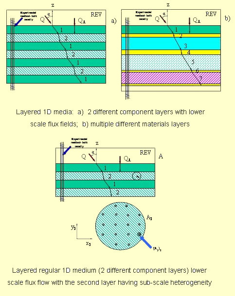
Taking the simplest combination of two phase composite of layered

or foamy, or using the foamy layers

structure, we have the averaged temperature of that composite to be modeled as

and mostly people expecting that the combined, bulk, average temperature equation can be modeled as

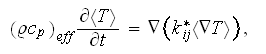
where the effective conductivity coefficient $k_{ij}^{\ast }$ is to be found somehow based on the composite's data - as phase' properties, morphology of composite arrangement, etc.

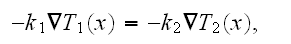
Combining the both temperature VAT equations ( if only two of phases are present) for the simplest case of constant coefficients (those are not such simple in a real protective shield medium)

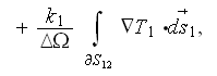
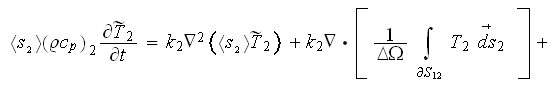
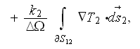
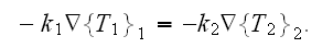
into one equation by adding one to another (when taking into account the boundary condition of temperature fluxes equality at the interface surface - )

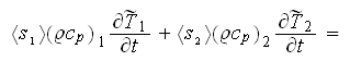
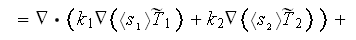
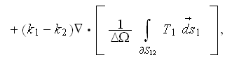
we get the strange equation which has the three different temperatures - $\widetilde{T}_{1},$ and ?

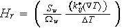
Still our goal is not to solve this strange equation, but - to reduce the rate of the heat flux (in another words, the overall amount of heat transported through the wall) of the composite 1D structure - the heat transfer rate per unit volume of protective wall per unit temperature difference $H_{r}$

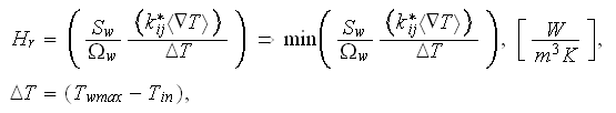
where $T_{wmax}$ is the hot side wall temperature, $T_{in}$ is the cold (other) side reference temperature, and of its intensity $I_{r}$

Unfortunately, we need to solve the both problems - the two-scale HSP-VAT heat conductivity problem via the composite protective wall, as well as the optimization (minimization) of the heat transfer rate problem. If we would now have the formulae for the Effective coefficient of conductivity, the both problem would be easier to solve.

That is not the case and because of this the optimization (minimization) of the heat transfer rate problem is continue to be the "UNSOLVED PROBLEM" now even for the constant coefficients statement. The few reasons for difficulties are:

a) this is the two-scale HSP-VAT problem, no matter what people ARE SOLVING AND SAYING RIGHT NOW;

b) this is the distributed parameters optimization problem with the aggravated mathematical statement of the Two-Scale problem, and not a single of these optimization problems was solved up to these days;

c) this is the problem with the Heterogeneous Transient two phase effective coefficients.

To find out the effective coefficient of conductivity for the composite two-phase medium as for the phase constand coefficients

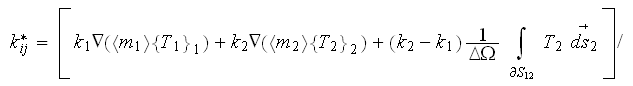
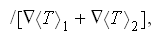
one still needs to solve the HSP-VAT two-scale problem first. The nonlinear heat conductivity HSP-VAT problem in a two-phase composite involves the definition for the effective coefficient of conductivity

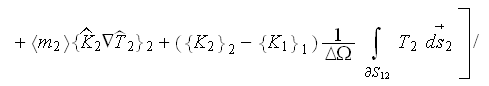
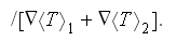
And by the way, in all these developments the transient effective coeficients $k_{ij}^{\ast },$ $K_{ij}^{\ast }$ are still not exact match to the one temperature homogeneous equation equation

The problem is with the left hand side governing equation forms, they are not identical, they need to be matched one to another.

So, the heat transfer rate minimization brings in the complicated two-phase coefficient of conductivity assessment. We have done this kind of assessment for the semiconductor heat sink two-scale solution and optimization see in -

- "Heat Exchangers,"

- "Semiconductor Coolers"

- and - "Further Reading and Consulting".

As we have shown in the - "When the 2x2 is not going to be 4 - What to do?".

the problem which itself presents the basis for design of protective thermal barrier and which was considered during at least the last 70-80 years as the one that had been solved finally and completely, and in a linear form as being solved exactly analytically, but in reality it was not.

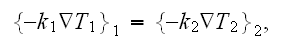
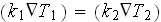
It even can not be solved with the one scale homogeneous physics mathematical statement, because it has the discrepancy features those can not be explained within the one scale mathematical statement, for example, according to homogeneous statement the equality for heat fluxes in each of the layers

should be preserved with the temperature fields found in the solution for the averaged fluxes

as soon as in homogeneous physics

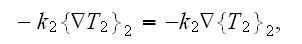
then should be

But this equality does not happen, so why? and What does it mean?

Recently this problem has been solved as the two-scale HSP-VAT mathematical formulation. What is interesting is that it can be solved for a linear case (with the constant phase coefficients) in the strict analytical form, giving no chances for conventional treatment of this problem.

This also means that the thermal barrier (shield) problem design - on the each scale level, can not be found in brackets of the one scale treatment. The one scale design of the two- or three scale problem is not a valid design!

With this solution in mind it is interesting observing the properties of the found effective coefficient of conductivity.

If anyone asked himself (herself) - Why the problem with the starting conductivity coefficients ratio as high as with the good intention to decrease the total effective wall's thermal conductivity coefficient playing down the high value of one of the phase involved $k_{2}=90.0$ to $k_{2}=0.9,$ or for two orders of magnitude lower, and then still getting the result for the effective wall coefficient decreasing to a value only less than a two times smaller?

That's seems illogical ? What is the physical, and mathematical explanation of this fact? The problem is the straightforward one, no nonlinearity, no hidden difficulties in the solution, so why the final change for the $k_{eff}^{\ast }$ is so small? Or, better to say - Why the starting effective coefficient is so low?

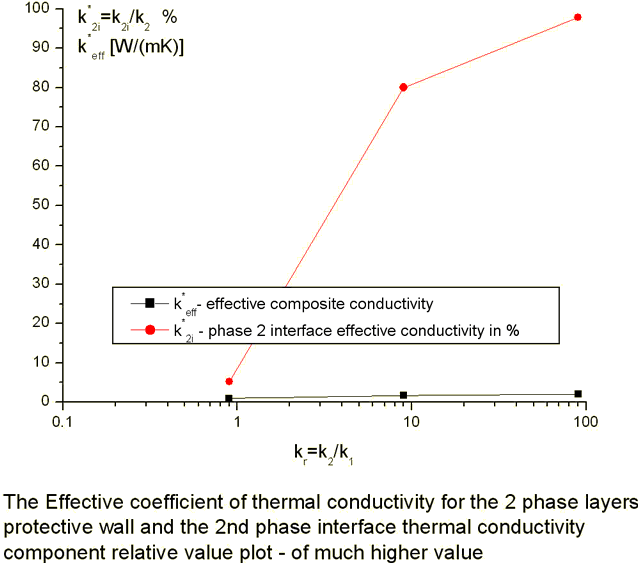
No answer to this question can be found in textbooks.

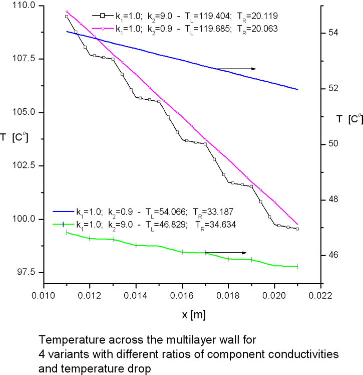
On the other hand - that is definitely more close to explanation when someone would watch the plots like this one

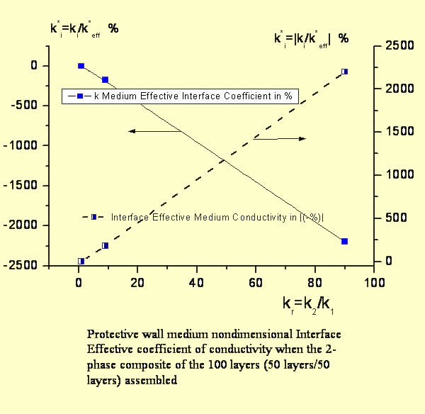
where based on HSP-VAT calculations the cause we have shown is of that as soon as there is some interface physical effect for the transport - which we call the interface effective (collective if you mind) conductivity coefficient which is actually going down and down in negative to balance in its specific way - by -177.8% of the final effective conductivity magnitude (for example, for the pair k₂=9.0, k₁=1.0), then the quantity of effective conductivity goes to the merely one quantity which is close to the lowest conductivity phase value.

See more explanations and detail in - "When the 2x2 is not going to be 4 - What to do?".