We will show in this subsection - What solution is considered usually and what methods used when the Wave Scattering problem in Acoustics (and some Electrodynamics problems) being stated as the one scale problem ?
As the goal here is the discussion and placing some comments on the problem of scattering, but not having a review in this field. We can select few characteristic examples of publications. One is of known and used often analysis is the review by Barabanenkov et al. (1971) (Barabanenkov, Yu.N., Kravtsov, Yu.A., Rytov, S.M., and Tamarskiï, V.I., (1971) , "Status of the Theory of Propagation of Waves in a Randomly Inhomogeneous Medium," Sov. Physics Uspekhi, Vol. 13, No. 5, pp. 551-575).
This is the pretty old review. Nevertheless, it can be used to set up a tone to what is considered as methods in scattering science (many physical fields have similar problems related to setting-up a method for wave scatteging in media of interest - thus, often the scattering of acoustics and EM waves are identical in linear statements) meaning acoustical, electromagnetic and many elastic problems.
On the first page - page 551 one can read:
"Propagation of waves in randomly-inhomogeneous media is such a vast field that we considered it expedient to limit our treatment only to problems of volume scattering in continuous media during free propagation.
Thus, we do not touch upon reflection at randomly-uneven surfaces, nor upon scattering by discrete inclusions, such as artificial scatterers, aerosols, raindrops, and snow in the atmosphere, or by bubbles or fish in the water, nor propagation of waves in randomly-inhomogeneous feeders.
However, even with these restrictions, the problems of both the theory itself and of its applications remain extremely varied. ..."
In this way authors told that they did not include directly the Heterogeneous Media treatments into their review. But actually the media models they explore embrace and the Heterogeneous media types.
And on page 552:
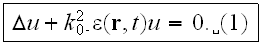
''To speak of posing the problem, in principle it involves a\underline{ stochastic wave equation}. Of course, in a number of cases the equations can be more complex than the Helmholtz equation. They can contain not only the second, but also the first derivatives of the wave field. They can be vector equations and form a system of simultaneous equations, as with electromagnetic waves or elastic waves in a solid.
However, the main thing, which is characteristic even in the simplest case of
a scalar wave equation, is that it involves a parametric equation, even if
only a linear one: the random functions of position and time that describe the
fluctuations in the properties of the medium do not enter additively, as
"external forces," but as coefficients in the equation itself. If, for
example, the time variations in the medium are so slow that we can take
account of them in a quasi-steady-state manner, then with a monochromatic
source (primary wave), the wave equation will be
The random "dielectric constant"
![]()
 enters here as a coefficient for the sought wave function
![]()
 This is the root of all the mathematical difficulties of the theory, since we
don't know how to find an exact solution of such a wave equation."
This is the root of all the mathematical difficulties of the theory, since we
don't know how to find an exact solution of such a wave equation."
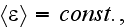
Page 552 - "..we shall assume for simplicity that the medium is on the average
homogeneous and stationary,
![]()
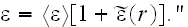
 while the fluctuations are quazistatical, i.g.,
![]()
The main method which stands behind almost all the scattering theories in many sciences is that.
Page 553 - "If
![]()
 is small enough, then we can naturally resort to the method of perturbations,
and expand
is small enough, then we can naturally resort to the method of perturbations,
and expand
![]()
 in a power series in
![]()
 or more exactly, in
![]()
 .
If we write (1) in the form
.
If we write (1) in the form
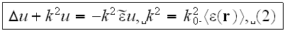
and use the Green's function for a homogeneous medium
![]()
 we can represent (2) as an integral equation
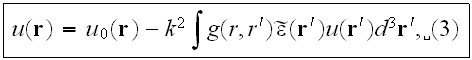
Here
![]()
 is the primary field that would have propagated in the medium in the absence
of fluctuations. By solving (3) by iterations, we get the perturbation-theory
series
is the primary field that would have propagated in the medium in the absence
of fluctuations. By solving (3) by iterations, we get the perturbation-theory
series
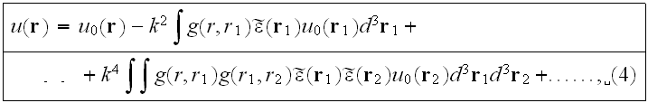
The n-th term of the series describes n-fold scattering, and contains the
n-fold product
![]()
 inside of n-fold integral. Thus, even in calculating
![]()
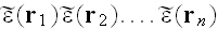
 we have to know the moments
![]()
 of
of
![]()
 of all orders.
However, under certain conditions that we shall discuss below, we can restrict
ourselves to the first (after
![]()
 term of the series. This is the single-scattering approximation, which even
Rayleigh had used in optical problems, and which is often called the Born
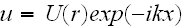
approximation in quantum mechanics. In this approxiamtion, the amplitude
term of the series. This is the single-scattering approximation, which even
Rayleigh had used in optical problems, and which is often called the Born
approximation in quantum mechanics. In this approxiamtion, the amplitude
![]()
 of the primary field does not decline as it penetrates deeper into the medium
(extinction is ignored), while the scattered field depends linearly on
of the primary field does not decline as it penetrates deeper into the medium
(extinction is ignored), while the scattered field depends linearly on
![]()
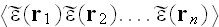
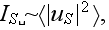
 Hence, in order to calculate the correlation function
![]()
 of the scattered field, and particularly, its intensity
![]()
 it suffices to know the correlationfunction of
![]()
 i.g.,
i.g.,
![]()
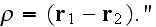
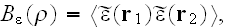 where
where
![]()
This means the talk is about the LOCAL FIELDS SCATTERING Problem solution. This is not about the Upper scale field description.
"The Born approximation proves quite sufficient in very many problems, not only a scalar, but also for an electromagnetic field."
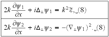
Among wildely used methods for the Large-Scale inhomogeneities described shortly are "parabolic equation method (PEM), the method of smooth perturbations (MSP), and the Markov Approximation.
Scattering by Large-Scale Inhomogeneities
Parabolic Equation Method
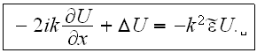
Page 554 - " If we assume in eq. (1) that
![]()
 ,
wherethe x coordinate is defined by the direction of propagation of the
primary wave, we get the following equation for the complex amplitude
,
wherethe x coordinate is defined by the direction of propagation of the
primary wave, we get the following equation for the complex amplitude
![]()

If
![]()
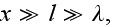 then
then
![]()
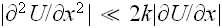 (of the order of
![]()
 Then we can replace the total Laplacian
![]()
 by the transverse Laplacian
![]()

![]()
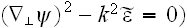
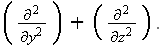 This leads to the parabolic equation
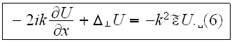
In using eq. (6), people often speak of the differential approximation. The
source of this terminology is evident from the form of the left-hand side
(although the diffusion coefficient is imaginary, as it is in the Schrodunger
equation), and the physical meaning consists in a slow transverse diffusion of
the energy of the wave field with increasing
![]()
 ."
."
Method of Smooth Perturbations (MSP)
page 554 - "The method of smooth perturbations (MSP) is distinguished by the
fact that one introduce the complex phase
![]()
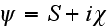 i place of
![]()
 .
Here
.
Here
![]()
 is the phase proper, while
![]()
 is the logarithm of the amplitude, or the so-called level. Substituting
![]()
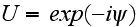 into (6) get the fundamental MSP equation:
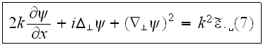
In contrast to (6), it is no longer parametric, but instead, in non-linear.
The Green's function of te left-hand sides of the parabolic equation (6) and
the linearized eq. (7) (i.g., eq. (6) with
![]()
 and eq. (7) with
![]()
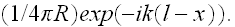
 correspond to the so-called parabolic or Fresnel approximation:
![]()
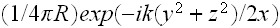 replaces the exact function
![]()
"Consequently, one must also resort here to the procedure of perturbations and rely on the smallness of the fluctuations."
Page 555 - "Expansion of the complex phase in the series
![]()
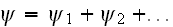 ,
where in of the order of
,
where in of the order of
![]()
 ,
gives rise to a system of linear equations of successive approximations
,
gives rise to a system of linear equations of successive approximations
The right hand side of these equations rapidly become more complicated with
increasing n. Just as in the Born approximation, one naturally considers first
the problem of the conditions under which one can limit the treatment to the
first approximation
![]()
 ."
."
Here we should note - and that the reader also should note - How many assumptions were put here just to solve the approximate problem?
Now it is the time to move to the Multiple Scattering.
Page 561 - "The general theory of multiple scattering has been developed in the last seven years."
That was the publcation of 1971 !
"During this time, the Green's-function method, which had previously been
developed in quantum electrodynamics, was applied to the discussed macroscopic
problems. To speak more ..., people have used the Dyson
equation![]()
![$^{[459]}$](/acoustics/pic/scatteringacous__52.gif) for the mean field
for the mean field
![]()
 and the Bethe-Salpeter
equation
and the Bethe-Salpeter
equation![]()
![$^{[460]}$](/acoustics/pic/scatteringacous__54.gif) for the covariance
for the covariance
![]()
 or the correlation function
![]()
 These equations were derived by using the graph technique of
Feynman.
These equations were derived by using the graph technique of
Feynman.![]()
![$^{[457,458]}$](/acoustics/pic/scatteringacous__57.gif) Thus it is again a question of deriving equations
for averaged quantities.
However, one can not derive closed equations of this
type by averaging the original differential equations for the field
Thus it is again a question of deriving equations
for averaged quantities.
However, one can not derive closed equations of this
type by averaging the original differential equations for the field
![]()
 because of their parametric nature: the moments of different orders
are coupled
together." - this text is highlighted here.
because of their parametric nature: the moments of different orders
are coupled
together." - this text is highlighted here.
At this place we need to put a couple of notes: First of all - the statement about "one can not derive closed equations of this type by averaging the original differential equations" is wrong; and 2) that was the publication, the approach with these Dyson (D.) equation and the Bethe-Salpeter (B.-S.) equation - this text was written all above the 25 years before the VAT theorems and the averaging techniques find the way into the acoustics and electrodynamics areas; 3) And again - 'the original differential equations" here in Scattering acoustics and Optics are and were constructed on the base of Boltzmann's equation - which is itself incorrect.
"Hence, one must resort to solving (4), although it is wtitten in the form of a perturbation-theory series. The graph technique makes it possible formally to sum this series, as well as the product of two such series, and this leads to the Dyson (D.) equation and the Bethe-Salpeter (B.-S.) equation."
It's interesting what is written there on the Boltzmann equation - so often used as a "first-principles" equation.
"People had also encountered multiple scattering long ago in the problem of
passage of radiation through the atmospheres of stars and
planets,![]()
![$^{[461-466]}$](/acoustics/pic/scatteringacous__59.gif) and in problems of scattering of thermal
neutrons,
and in problems of scattering of thermal
neutrons,![]()
![$^{[467,468]} $](/acoustics/pic/scatteringacous__60.gif) charged
particles,
charged
particles,![]()
![$^{[469]}$](/acoustics/pic/scatteringacous__61.gif) etc. Here they usually used the linearized integro-differential equation of
Boltzmann. In view of the classicaldescription of motion of particles or
radiation along trajectories (rays) (i.e., description in the geometrical
optics approximation), this equation is a so-called transport equation (of
particles of energy). Typically, of coarse, wave-interference effects are not
taken into account here."
etc. Here they usually used the linearized integro-differential equation of
Boltzmann. In view of the classicaldescription of motion of particles or
radiation along trajectories (rays) (i.e., description in the geometrical
optics approximation), this equation is a so-called transport equation (of
particles of energy). Typically, of coarse, wave-interference effects are not
taken into account here."
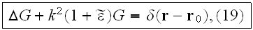
"What do the D. and B.-S. equations look like?
Let
![]()
 be the sought Green's function, i.e., a solution of the following equation
that satisfies the condition of radiation to infinity:
be the sought Green's function, i.e., a solution of the following equation
that satisfies the condition of radiation to infinity:
and, as before, let
![]()
 be the Green's function in a homogeneous medium
![]()
 The D. equation for
![]()
 is
is

![]()
 in symbolic (operator) form,
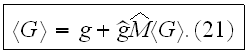
Here the "kernel"
![]()
 ,
which is called the "polarization operator", is an infinite series, being the
sum of the so-called strongly connected graphs having no external propagation
lines.
,
which is called the "polarization operator", is an infinite series, being the
sum of the so-called strongly connected graphs having no external propagation
lines.
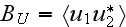
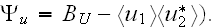
The B.-S. equation has an analogous form. For the mixed moment
![]()
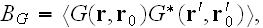 it can be written as follows:
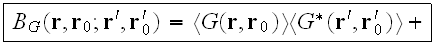
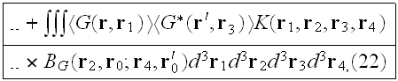
or, in operator form:
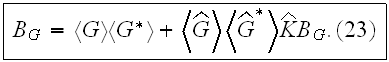
It contains as a "kernel" the intensity operator K..... which depends on four arguments, and it also a sum of strongly connected, but two-row graphs having no external propagation lines. Superficially, the two equations look like linear integral equations, but actually this isn't so. The "kernels" M and K are infinite series whose summation cannot actually be carried out."
Page 563 - "Then what is the worth of these equations?
First, they help in studying a number of the general problems of the theory of multiple scattering: in linking the problems of continuous randomly-inhomogeneous media and of sets of discrete scatterers (which we are not treating here), in revealing the various approximate approaches and elucidating the relation between them, and in particular, in providing a basis for the transport equation (see below).
Second, they become an actual means of solving concrete problems whenever one can replace the "kernels" M and K with approximate (abbreviated) expressions, i.e., known functions of the coordinates. Then, the D. and B.-S. equations become linear integral equations that can be solved under certain supplementary assumptions."
And final message on page 566 includes:
"In estimating the current status of the theory of volume scattering as a whole, we can state that, in spite of the substantial growth of the general theory of multiple scattering, the most productive methods from the standpoint of concrete results are still the original methods: the method of small perturbations, the MSP, and the PEM. Among the assets of the general theory of mutiple scattering we can list that it provides a basis for the transport equation."
The things had been moved since that paper as, for example, Turner and Weaver (1994) reported on the development of D. and B.-S. equations via the "ensemble average."
Ishimaru (1978b) gave the description of theory of the "first order smooting approximation for the Dyson equation". We will follow that exposition.
On the page 253 we can read - "The diagram method gives a systematic and concise formal representation of the complete multiple scattering processes based on an elementary use of Feynman diagrams (Frisch, 1968; Marcuvitz, 1974; Tatarski, 1971, Chapter 5). This leads to the diagram representation of the Dyson equation for the average field and the Bethe-Salpeter equation for the correlation function.
It is noted, however, that it is impossible to obtain the explicit exact expressios of the operators in these integral equations, and it is necessary to resoty to approximate representations. The simplest and the most useful is called the first order smoothing approximation. This approximation can be shown to be equivalent to the Twersky integral equations (Ishimaru, 1975)."
Page 254 - "14-1 MULTIPLE SCATTERING PROCESS CONTAINED IN TWERSKY'S THEORY"
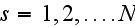
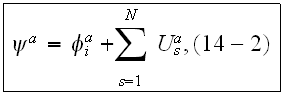
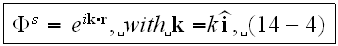
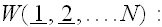
If we consider a random distribution of N particles located at spots
![]()

![]()
 in a volume V. These particles can be different in shape and size. The linear
wave equation for a field
in a volume V. These particles can be different in shape and size. The linear
wave equation for a field
![]()
 in a "fluid" (matrix) space not occupied by particles-scatterers is written as
where
![]()
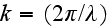 is the wave number of the "fluid" medium surrounding the particles. The
function
is the wave number of the "fluid" medium surrounding the particles. The
function
![]()
 is the incident wave function when there is no particles at point
![]()
 Then the field
![]()
 at
at
![]()
 is the sum of the incident wave
![]()
 and the scattering contributions
![]()
 from all N particles around located at points
![]()

![]()
NOTE - we stop talking here about particles as particles and accept them as point-like objects. This is Elimination of the Second Phase presented in the problem.
The
"![]()
 named for the wave at
![]()
 scattered from the scatterer located at
![]()
 and can be expressed in terms of the wave
![]()
 incident upon the scatterer at
![]()
 and the scattering characteristic
![]()
 of the particle located at
![]()
 as observed at
![]()
 so,
we write the linear formula
so,
we write the linear formula
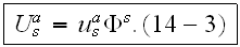
Note - that the scattering characteristic
![]()
 has the usual meaning of a functional characterisitic.
"Note that, in deneral,
![]()
 does not mean the product of
![]()
 and
and
![]()
 It is the only a synbolic notation to indicate the field at
![]()
 due to the scatterer at
![]()
 when the wave
![]()
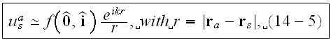
 is incident upon it. Only when
![]()
 can be approximated by a plane wave propagating in the direction of a unit
vector
can be approximated by a plane wave propagating in the direction of a unit
vector
![]()

and when the distance between
![]()
 and
and
![]()
 is large, we can use the following far field approximation of
![]()

where
![]()
 is a unit vector in the direction of
![]()
 and
and
![]()
 is the scattering amplitude of the scatterer."
The wave
![]()
 incident upon the scatterer at point
![]()
 is the "effective" field. This wave is the sum of the incident wave
![]()
 at point
![]()
 and
the waves scattered from all particles surrounding this one at
and
the waves scattered from all particles surrounding this one at
![]()

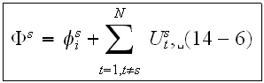
Equations (14-2) and (14-6) become equations
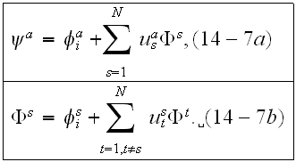
"In principle we can eliminate
![]()
 from these two equations and obtain the solution
![]()
 for a given incident wave
![]()

Note - that the waves
![]()
 are not directly tied to the wave equations.
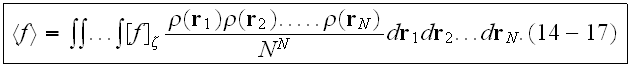
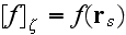
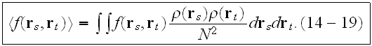
Page 259 - "Let us consider a random function f which depends on all
![]()
 scatterers. It may be a field quantity
![]()
 or a product of field quantities. We consider the ensemble average of this
function
or a product of field quantities. We consider the ensemble average of this
function
![]()
 .
The average is given in terms of a probability density function
.
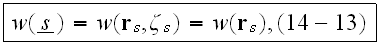
The average is given in terms of a probability density function
![]()

The variable
![]()
 designates all the characteristics of the scatterer s such as location
![]()
 shape, orientaion, and dielectric constant. Therefore, we may write
![]()
 where
where
![]()
 designates the volume
![]()
 integral
![]()
 and
and
![]()
 represents all the other characteristics of the scatterer:

Now we consider an important case in which the particle density is low and the particle size is much smaller that the separation between particles. In this case, we can neglect the finite size of particles and we can assume that the location and characteristics of each scatterer are independent of the locations and characteristics of other scatterers. This also means that all particles are considerd as point particles," (emphasized by us).
"and the effect of size appears only in scattering characteristics. Under
this assumption, we have

Next, we assume that all scatterers have the same statistical characteristics.
Then writing
we can perform integration with respect to all the characteristics
![]()
 Thus, we get
![]()


wher
![]()
 represents the average of
![]()
 corresponding to the average charcteristics of the scatterer (shape,
orientation, etc.)."
corresponding to the average charcteristics of the scatterer (shape,
orientation, etc.)."
This is the another great Assumption.
Again, there is no Field presented which would be described by differential Wave Governing Equations !!
"The probability density function
![]()
 may be interpreted as follows:"
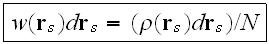
where
![]()
 is the "number density," then
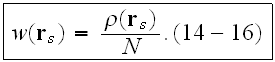
Then the averaged function can be written as
"If
![]()
 depends only on the location of the scatterer(s) and not on the location of
other scatterers, then writing
depends only on the location of the scatterer(s) and not on the location of
other scatterers, then writing
![]()
 ,
we integrate
,
we integrate
![]()
 over all
![]()
 except
![]()

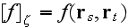
"If
![]()
 depends on the locations of two different scatterers s and t, then writing
![]()
 ,
we obtain
,
we obtain
And finally on the page 262 - " We note that this expanded form (14-25) is
identical to the Foldy-Twersky integral equation
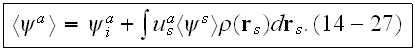
The equivalence between (14-25) and (14-27) can be established by iterating (14-27).
The integral equation (14-27) is the Basic Equation for the coherent field in Twersky's theory.
This equation was obtained by Foldy as an approximation,".... then Twersky determined that it has clearly established its physical means through an algorithm followed above.
Note - Of coarse, this is the Effective Field theory? This theory in other scientific disciplines-areas, is very much known as the insufficient one.
Another level of scattering approached in the paper by Lin and Raptis (1985)
"Three types of the problems are thoroughly considered:
1) scattering of the incident wave from rigid and stationary cylinders;
2) scattering of the radiated waves caused by the oscillations of the cylinders;
3) scattering of the incident wave from rigid and oscilatory cylinders. in each case the effect of multiple scattering is taken into account.''
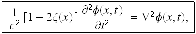
Interesting enough here is that the equations they used to calculate multiple
scattering from parallel cylinders are the homogeneous equations (the problem
stated as a homogeneous one)
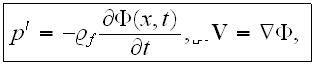
(they have an error - should be the sign - before r.h.s. in this equation),
where
![]()
 is the perturbed velocity potential of the fluid
![]()
 ,
,
![]()
 is the speed of sould in the undisturbed fluid,
![]()
 is the density of the unperturbed fluid.
''The boundary conditions are that:
1) the normal component of the fluid velocity at the boundary of the cylinder is equal to the vibrational velocity in that direction, and
2) the scattered and radiated waves must be outward traveling.
Written explicitly, the boundary condition at the surface of cylinder
![]()
 is
is
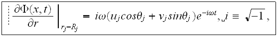
where
![]()
 is the radius of cylinder
![]()

![]()
 and
and
![]()
 are the displacement amplitudes in the x and y directions, and
![]()
 is
the oscillation frequency.''
is
the oscillation frequency.''
The method, results and their description can be useful if providing the same or close in physics problem.
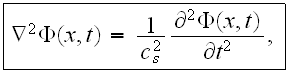
In Sato's (1982) paper used for description of scalar waves
![]()
 in three-dimensional inhomogeneous media the equation
where
![]()
 is the mean velocity of sound and
![]()
 is the fractional velocity fluctuation.
Reference exists to the Chernov's book, where is the Born's approximation used.
CONCLUSIONS
The body of texts on scattering in this subsection openly votes for the statement that the theory and methods are meant and used for the one phase one scale local field values. Even when problem stated as with the Dyson equation.
There is the list of serious assumptions into this developed traditional science of one scale scattering. We won't enumerate all of them - but one, which is the particularly appealing - that the other, the second phase (if only of two phases medium consists) the scattering media described by nothing but algebraic or functional characteristics. There are no mathematical physics governing equations for the second phase scattering medium.
So, mostly this means - We Have the One Field Problem when addressing the two- (or more) phase problem in wave scattering. Isn't it interesting?
To treat the scattering problem in the whole continuum space - there was invented the concept - that the medium is the inhomogeneous continuous space with the characteristics which are inhomogeneous in space. That's true to some extent, meanwhile the most of media are the Heterogeneous media type, not Inhomogeneous.
References
Barabanenkov, Yu.N., Kravtsov, Yu.A., Rytov, S.M., and Tamarskiï, V.I., (1971), "Status of the Theory of Propagation of Waves in a Randomly Inhomogeneous Medium," Sov. Physics Uspekhi, Vol. 13, No. 5, pp. 551-680.
Barabanenkov, Yu.N., Kravtsov, Yu.A., Ozrin, V.D., and Saichev, A.I., (1991), "Enhanced Backscattering in Optics," chap. 2 in Progress in Optics, Vol. XXIX, E.Wolf, ed., Elsevier Science Publ., Amsterdam, pp. 64-197.
Chernov, L.A. Wave Propagation in Random Media, McGraw-Hill, New York, 1960. 168 p.
Ishimaru, A., Wave Propagation and Scattering in Random Media, Academic Press, New York, Vol. 1, 1978a. 255p.
Ishimaru, A., Wave Propagation and Scattering in Random Media, Academic Press, New York, Vol. 2, 1978b. 253-572pp.
Lin, W.H. amd Raptis, A.C., (1985), "Sound Scattering by a Group of Oscillatory Cylinders," J. Acoust. Soc. Am., Vol. 77, No. 1, pp. 15-28.
Malyshkin, V., McGurn, A.R., Elson, J.M., and Tran, P., "Transverse or Off-axis Localization of Electromagnetic Waves in Random One- and Two-Dimensional Dielecric Systems Which are Periodic on Averaged," Waves in Random Media, Vol. 8, No. 2, pp. 203-228, 1998.
Sato, H., (1982), "Amplitude Attenuation of Impulsive Waves in Random Media Based on Travel Time Corrected Mean Wave Formalism," J. Acoust. Soc. Am., Vol. 71, No. 3, pp. 559-564.
Soukoulis, C.M., ed., Photonic Band Gaps and Localization, Plenum, New York, 1993.
Soukoulis, C.M., ed., Photonic Band Gap Materials, Kluwer Academic Publishers, Dordrecht, 1996. 729 p.
Turner, J.A. and Weaver, R.L., "Radiative Transfer of Ultrasound," J. Acoust. Soc. Amer., Vol. 96, No. 6, pp. 3654-3674, 1994.
Turner, J.A. and Weaver, R.L., "Radiative Transfer and Multiple Scattering of Diffuse Ultrasound in Polycrystalline Media," J. Acoust. Soc. Amer., Vol. 96, No. 6, pp. 3675-3683, 1994.
Varadan, V.K., Ma, Y., and Varadan, V.V., "A Multiple Scattering Theory for Elastic Wave Propagation in Discrete Random Media," J. Acoust. Soc. Am., Vol. 77, No. 2, pp. 375- 385.
Varadan, V.K., Ma, Y., and Varadan, V.V., (Eds.), Acoustic, Electromagnetic and Elastic Wave Scattering - Focus on the T-Matrix Approach, Pergamon, New York, 1980.
Varadan, V.V., Lakhtakia, A., and Varadan, V.K., "Comments on Recent Criticism of the T-Matrix Method," J. Acoust. Soc. Am., Vol. 84, No. 6, pp. 2280-2284, 1988.